Robot Radio
The official radio documentation is complete and detailed, and should serve as your primary resource.
https://frc-radio.vivid-hosting.net/
However, It's not always obvious what you need to look up to get moving. Consider this document just a simple guide and jumping-off point to find the right documentation elsewhere
Setting up the radio for competition
You don't! The Field Technicians at competitions will program the radio for competitions.
When configured for competition play, you cannot connect to the radio via wifi. Instead, use an ethernet cable, or
Setting up the radio for home
The home radio configuration is a common pain point
Option 1: Wired connection
This option is the simplest: Just connect the robot via an ethernet or USB, and do whatever you need to do. For quick checks, this makes sense, but obviously is suboptimal for things like driving around.
Option 2: 2.4GhZ Wifi Hotspot
The radio does have a 2.4ghz wifi hotspot, albeit with some limitations. This mode is suitable for many practices, and is generally the recommended approach for most every-day practices due to ease of use.
Note, this option requires access to the tiny DIP switches on the back of the radio! You'll want to make sure that your hardware teams don't mount the radio in a way that makes this impossible to access.
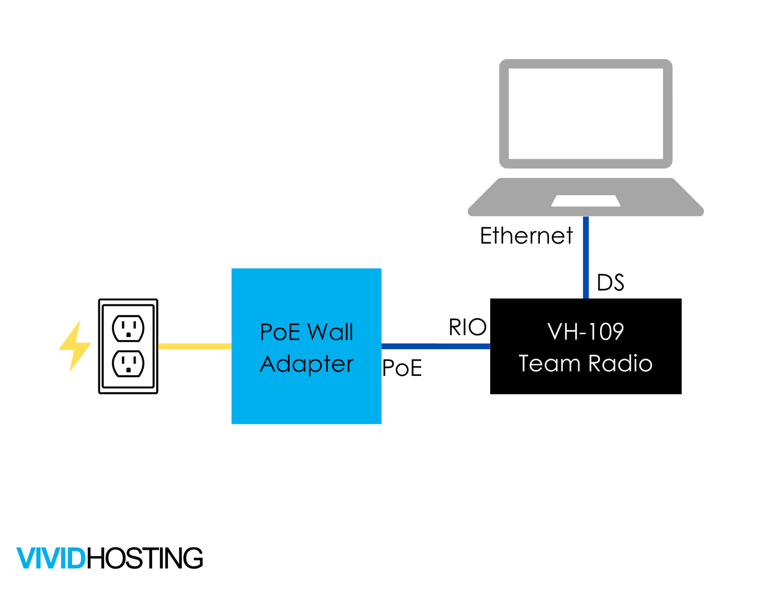
Option 3: Tethered Bridge
This option uses a second radio to connect your laptop to the robot. This is the most cumbersome and limited way to connect to a robot, and makes swapping who's using the bot a bit more tricky.
However, this is also the most performant and reliable connection method. This is recommended when doing extended driving sessions, final performance tuning, and other scenarios where you're trying to simulate competition-ready environments.
This option has a normal robot on one end, and your driver-station setup will look the following image. See https://frc-radio.vivid-hosting.net/overview/practicing-at-home for full setup directions
Bonus Features
Port Forwarding
Port forwarding allows you to bridge networks across different interfaces.
The practical application in FRC is being able to access network devices via the USB interface! This is mostly useful for quickly interfacing with Vision hardware like the Limelight or Photonvision at competitions.
//Add in the constructor in Robot.java or RobotContainer.java

// If you're using a Limelight
PortForwarder.add(5800, "limelight.local", 5800);
// If you're using PhotonVision
PortForwarder.add(5800, "photonvision.local", 5800);
Scripting the radio
The radio has some scriptable interfaces, allowing programmatic access to quickly change or read settings.
Basic Telemetry
Goals
Understand how to efficiently communicate to and from a robot for diagnostics and control
Success Criteria
- Print a notable event using the RioLog
- Find your logged event using DriverStation
- Plot some sensor data (such as an encoder reading), and view it on Glass/Elastic
- Create a subfolder containing several subsystem data points.
As a telemetry task, success is thus open ended, and should just be part of your development process; The actual feature can be anything, but a few examples we've seen before are
Why you care about good telemetry
By definition, a program runs exactly as you the code was written to run. Most notably, this does not strictly mean the code runs as it was intended to.
When looking at a robot, there's a bunch of factors that can have be set in ways that were not anticipated, resulting in unexpected behavior.
Telemetry helps you see the bot as the bot sees itself, making it much easier to bridge the gap between what it's doing and what it should be doing.
Printing + Logging
Simply printing information to a terminal is often the easiest form of telemetry to write, but rarely the easiest one to use. Because all print operations go through the same output interface, the more information you print, the harder it is to manage.
This approach is best used for low-frequency information, especially if you care about quickly accessing the record over time. It's best used for marking notable changes in the system: Completion of tasks, critical events, or errors that pop up. Because of this, it's highly associated with "logging".
The methods to print are attached to the particular print channels
//System.out is the normal output channel
System.out.println("string here"); //Print a string
System.out.println(764.3); //you can print numbers, variables, and many other objects

//There's also other methods to handle complex formatting....
//But we aren't too interested in these in general.
System.out.printf("Value of thing: %n \n", 12);
A typical way this would be used would be something like this:
public ExampleSubsystem{
	boolean isAGamePieceLoaded=false;
	boolean wasAGamePieceLoadedLastCycle=false;

	public Command load(){
		//Some operation to load a game piece and run set the loaded state
		return runOnce(()->isAGamePieceLoaded=true);
	}

	public void periodic(){
		if(isAGamePieceLoaded==true && wasAGamePieceLoadedLastCycle==false){
			System.out.print("Game piece now loaded!");
		}
		if(isAGamePieceLoaded==false && wasAGamePieceLoadedLastCycle==true){
			System.out.print("Game piece no longer loaded");
		}
		wasAGamePieceLoadedLastCycle=isAGamePieceLoaded
	}
}
Rather than spamming "GAME PIECE LOADED" 50 times a second for however long a game piece is in the bot, this pattern cleanly captures the changes when a piece is loaded or unloaded.
In a more typical Command based robot , you could put print statements like this in the end() operation of your command, making it even easier and cleaner.
The typical interface for reading print statements is the RioLog: You can access this via the Command Pallet (CTRL+Shift+P) by just typing > WPILIB: Start Riolog. You may need to connect to the robot first.
These print statements also show up in the DriverStation logs viewer, making it easier to pair your printed events with other driver-station and match events.
NetworkTables
Data in our other telemetry applications uses the NetworkTables interface, with the typical easy access mode being the SmartDashboard api. This uses a "key" or name for the data, along with the value. There's a couple function names for different data types you can interact with
// Put information into the table
SmartDashboard.putNumber("key",0); // Any numerical types like int or float
SmartDashboard.putString("key","value");
SmartDashboard.putBoolean("key",false);
SmartDashboard.putData("key",field2d); //Many built-in WPILIB classes have special support for publishing
You can also "get" values from the dashboard, which is useful for on-robot networking with devices like Limelight, PhotonVision, or for certain remote interactions and non-volatile storage.
Note, that since it's possible you could request a key that doesn't exist, all these functions require a "default" value; If the value you're looking for is missing, it'll just give you the provided default.
SmartDashboard.getNumber("key",0);
SmartDashboard.getString("key","not found");
SmartDashboard.getBoolean("key",false);
Networktables also supports hierarchies using the "/" seperator: This allows you to separate things nicely, and the telemetry tools will let you interface with groups of values.
SmartDashboard.putNumber("SystemA/angle",0);
SmartDashboard.putNumber("SystemA/height",0);
SmartDashboard.putNumber("SystemA/distance",0);
SmartDashboard.putNumber("SystemB/angle",0);
While not critical, it is also helpful to recognize that within their appropriate heirarchy, keys are displayed in alphabetical order! Naming things can thus be helpful to organizing and grouping data.
Good Organization -> Faster debugging
As you can imagine, with multiple people each trying to get robot diagnostics, this can get very cluttered. There's a few good ways to make good use of Glass for rapid diagnostics:
- Group your keys using
group/key. All items with the samegroup/value get put into the same subfolder, and easier to track. Often subsystem names make a great group pairing, but if you're tracking something specific, making a new group can help. - Label keys with units: a key called
angleis best when written asangle degree; This ensures you and others don't confuse it withangle rad. - Once you have your grouping and units, add more values! Especially when you have multiple values that should be the same. One of the most frequent ways for a system to go wrong is when two values differ, but shouldn't.
A good case study is an arm: You would have
- An absolute encoder angle
- the relative encoder angle
- The target angle
- motor output
And you would likely have a lot of other systems going on. So, for the arm you would want to organize things something like this
SmartDashboard.putNumber("arm/enc Abs(deg)",absEncoder.getAngle());
SmartDashboard.putNumber("arm/enc Rel(deg)",encoder.getAngle());
SmartDashboard.putNumber("arm/target(deg)",targetAngle);
SmartDashboard.putNumber("arm/output(%)",motor.getAppliedOutput());
A good sanity check is to think "if someone else were to read this, could they figure it out without digging in the code". If the answer is no, add a bit more info.
Glass
Glass is our preferred telemetry interface as programmers: It offers great flexibility, easy tracking of many potential outputs, and is relatively easy to use.
Glass does not natively "log" data that it handles though; This makes it great for realtime diagnostics, but is not a great logging solution for tracking data mid-match.
This is a great intro to how to get started with Glass:
https://docs.wpilib.org/en/stable/docs/software/dashboards/glass/index.html
For the most part, you'll be interacting with the NetworkTables block, and adding visual widgets using Plot and the NetworkTables menu item.
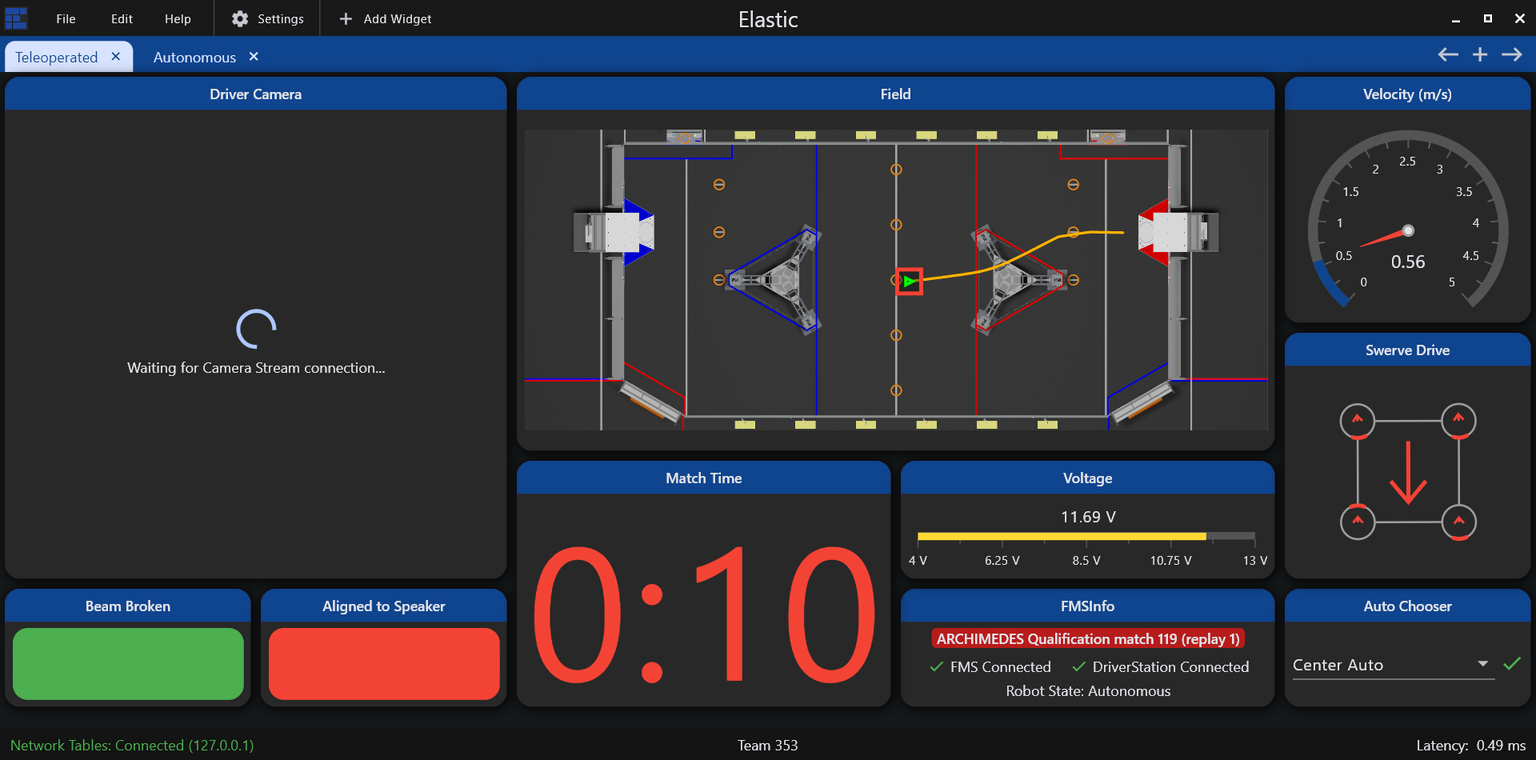
Elastic
Elastic is a telemetry interface oriented more for drivers, but can be useful for programming and other diagnostics. Elastic excels at providing a flexible UI with good at-a-glance visuals for various numbers and directions.
Detailed docs are available here:
https://frc-elastic.gitbook.io/docs
As a driver tool, it's good practice to set up your drivers with a screen according to their preferences, and then make sure to keep it uncluttered. You can go to Edit -> Lock Layout to prevent unexpected changes.
For programming utility, open a new tab, and add widgets and items.
Plotting Data
Motion Profiles
Success Criteria
- Configure a motion system with PID and FeedForward
- Add a trapezoidal motion profile command (runs indefinitely)
- Create a decorated version with exit conditions on reaching the target
- Create a small auto sequence to cycle multiple points
- Create a set of buttons for different setpoints
Synopsis
Motion Profiling is the process of generating smooth, controlled motion. This is typically done using controlled, intermediate setpoints, consideration of the system's physical properties, and other imposed limitations.
In FRC our tooling generally utilizes a Trapazoidal profile, allowing us precise control of system position, maximum system speed, and acceleration applied to the system.
Benefits of Motion profiling
Motion Profiling resolves several problems that can come up with "simpler" control systems such as simple open loop or straight PID control.
The first comes from acknowledgement of the basic physics equation
The next relates to "tuning": The process of adjusting robot parameters to generate consistent motion. If you've gone through the PID tuning process, you probably remember one struggle: Your tuning works great until you move the setpoint a larger distance, at which point it wildly misbehaves, and the system acts erratically. This case is caused by sharp changes in system error, resulting in the PID generating a large output. Motion profiles instead change the setpoint at a controlled rate, ensuring a small system error keeping the PID in a much more stable state.
The extra complexity is worth it! Tuning a system using a Motion Profile is significantly less work than without it, since all the biggest pain points are eliminated. Your PID behaves better, with no overshoot or sharp outputs, and your system
How it works
For these purposes, we're going to discuss a "positional" control system, such as an Elevator or Arm .
Motion Profiles still apply to velocity control Rollers and Flywheels; In those cases, we ignore the position, smoothly accelerating to our target velocity. This means we only see half the benefit on those systems.
The system we typically use is a "Trapezoidal" profile, named after the shape of the velocity graph it generates.
This system has just two parameters:
- A maximum velocity
- a maximum acceleration.
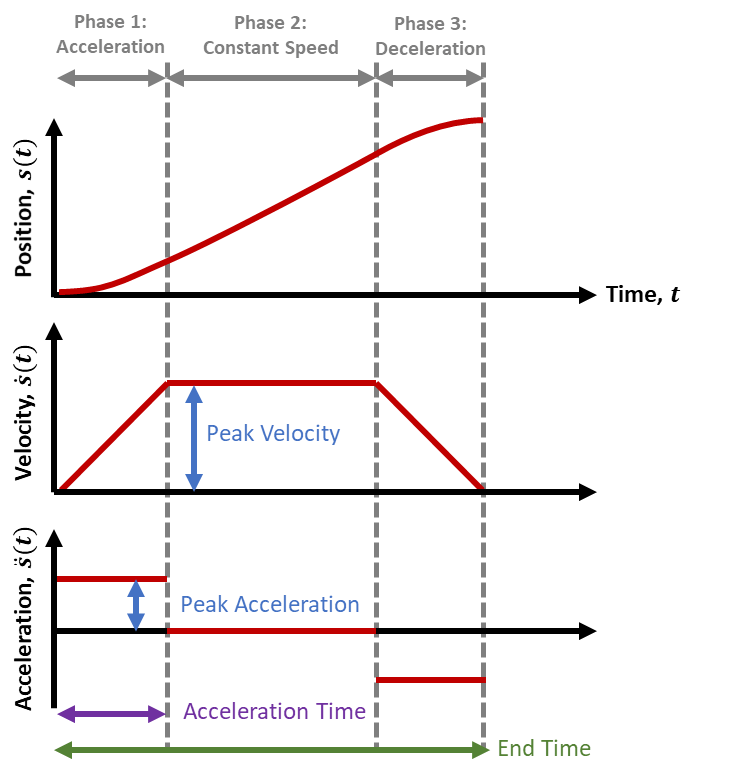
By having these values set at values the physical system can achieve, our motion profile can split up one large motion into 3 segments.
- An acceleration step, where the motor is approaching the max speed
- Running at our max speed
- Decelerating on approach to the final position.
Because our Motion Profile is aware of our system capabilities, it can then constrain our setpoint changes to ones that that our system can actually achieve, generating a smooth motion without overshooting our final target (or goal).
Since we know how long it takes to accelerate and decelerate, and the max speed, we can also predict exactly how long the whole motion takes!
The entire motion looks just like this:
Finding Max Velocity
A theoretical maximum can be found by multiplying your maximum motor RPM by your gear reduction: It's very similar to configuring your encoder conversion factor, then hitting it with your maximum velocity.
In practice, you normally want to start by setting it slow, at something that you can visually track: Often ~1-2 seconds for a specific range of motion. This helps with testing, since you can see it work and mentally confirm whether it's what you expect.
As you improve and tune your system, you can simply then increase the maximum until your system feels unsafe, and then go back down a bit.
In many practical FRC systems, you may not hit the actual maximum speed of your system: Instead, the system well simply accelerate to the halfway point and then decelerate. This is normal, and simply means the system is constrained by the acceleration.
Finding Max Acceleration
The maximum acceleration effectively represents the actual force we're telling the motor to apply. It's easiest to understand at the extremes:
- When set to zero, your system will never have force applied; It won't move at all.
- When set to infinite, your system assumes it can reach to the max velocity instantly; This is effectively just applying as much force as your system is configured for.
However, in actual systems you want them to move, so zero is useless. And infinite is useful, but impractical: Thinking back to our equation,
This final form helps us clearly see we have a maximum: Our output force is is defined by the motor's max output and our system's mass, giving us a maximum constraint:
Note this is highly simplified: Actually calculating max acceleration this way on real-world systems is often non-trivial, and involves significantly more variables and equations than listed here. However, it's the concept that's important.
In practice, the easiest way to find acceleration is to simply start small increase the acceleration until the system moves how you want. If it starts making concerning noises or over-shooting, then you've gone too far, and you should back it off.
Revisiting the graph
With some background, there's a couple ways to visually interpret this graph:
- This graph always represents the generated profile, but also should reflect your actual position too! When configured correctly, the generated graph is always within our system's capability.
- The calculated "position" setpoint is generally what we feed to our system's PID output.
- The "acceleration" impacts the angle on our velocity trapezoid! At infinite, it's vertical, and at zero, it's horizontal.
Interactions with FeedForwards
Having a motion profile also enables inputs for FeedForwards, allowing even higher levels of precision on your expected outputs.
At the basic level, positional PIDs can be trivially configured with kG and kS, which only depend on values known on all systems. kG is constant or depends on position, and kS depends only on direction of motion.
However, the kV and kA gains both depend on not just on position, but also a known system acceleration and velocity targets.... which we haven't had with arbitrary setpoint jumps.
But now, we can plan our motion: Giving us velocity and acceleration targets. With the right feedforwards, we can now compute the moment-to-moment output for the entire motion in advance!
Interaction with PIDs
The most important part is that our error changes from one big setpoint jump to a lot of small, properly calculated ones.
Without a feed-forward, simply having a motion profile completely removes the big transitions and associated output spikes. This makes tuning simpler, less critical, and often allows for more aggressive PID gains without problems. However, many positional systems will usually still need an I term to accurately hit setpoints accurately without rapid oscillations from a high P term.
With a partial FeedForward (kG + kS) the Feed-Forward handles the base lifting, reducing the need of a PID to handle gravity. This leaves the PID left to handle the motion itself, and it can easily hit setpoint targets without an I term, barring weight changes (such as loaded game pieces)
With a full FeedForward, the error between commanded motion and actual motion will be extremely small, making the PID's impact almost completely irreverent. This makes the PID tuning extremely easy, and the gains can be tuned for precisely the expected disturbances you'll encounter, such as impacts or weight variation.
Note, that despite having theoretically minimal impact, you would still always want a PID to ensure the system gets back to position in cause of error.
Tuning Errors and Adjustments
Fortunately, with motion profiles you get a lot, with very little in the way of potential problems.
Most errors can be easily captured by looking at the position and velocity graph of a real system, and applying a bit of reasoning on what line isn't matching up.
- Overshooting the position setpoint at the end: This likely means your acceleration is too high, or your I gain is too large.
- The system is lagging behind the setpoints and the lines are diverting entirely. It then overshoots the setpoint: Your system cannot output enough power to meet your acceleration constraint. Make sure you have appropriate current limits, and/or lower the acceleration within the system capability.
- The system is lagging behind the setpoints so the lines are parallel but offset: This is typical when not using kA+kV, or when they're set too low. The difference is how long it takes the PID control to kick in and make up for what kA+kV should be generating for that motion.
- The motion is very jerky when travelling at the max speed: This usually means kV is too high, but can be kS being too high. Lowering kP may help as well.
- It starts really awful and smooths out: Likely kA is too high, although again kS and kP can influence this.
Implementing <system type here>
The full system and example code is part of the system descriptions:
The most effective way in general is using the WPILib ProfiledPIDController providing the simplest complete implementation.
This works as a straight upgrade to the standard PID configuration, but takes 2 additional parameters that grant huge performance gains and easier tuning.
ExampleElevator extends SubsystemBase{
	SparkMax motor = new SparkMax(42,kBrushless);
	//Configure reasonable profile constraints
	private final TrapezoidProfile.Constraints constraints =
		new TrapezoidProfile.Constraints(kMaxVelocity, kMaxAcceleration);
	//Create a PID that obeys those constraints in it's motion
	//Likely, you will have kI=0 and kD=0
	//Note, the unit of our PID will need to be in Volts now.
	private final ProfiledPIDController controller =
		new ProfiledPIDController(kP, kI, kD, constraints, 0.02);
	//Our feedforward object appropriate for our subsystem of choice
	//When in doubt, set these to zero (equivilent to no feedforward)
	//Will be calculated as part of our tuning.
	private final ElevatorFeedforward feedforward =
		new ElevatorFeedforward(kS, kG, kV);

	//Lastly, we actually use our new
	public Command setHeight(Supplier<Distance> position){
		return run(
		()->{
			//Update our goal with any new targets
			controller.setGoal(position.get().in(Inches));
			//Calculate the voltage
			voltage=
			motor.setVoltage(
				controller.calculate(motor.getEncoder().getPosition())
				+ feedforward.calculate(controller.getSetpoint().velocity)
			);
		});
	}
The big difference compared to our other, simpler PID is that we're using motor.setVoltage for this; This relates to the inclusion of FeedForwards which prefers volts for improved consistency as the battery drains.
While the PID itself doesn't care, since we're adding them together they do need to be the same unit.
If you already calculated your PID gains using motor.set() or
Homing Sequences
Homing is the process of recovering physical system positions, typically using relative encoders.
Part of:
SuperStructure Arm
SuperStructure Elevator
And will generally be done after most requirements for those systems
Success Criteria
- Home a subsystem using a Command-oriented method
- Home a subsystem using a state-based method
- Make a non-homed system refuse non-homing command operations
- Document the "expected startup configuration" of your robot, and how the homing sequence resolves potential issues.
Lesson Plan
- Configure encoders and other system configurations
- Construct a Command that homes the system
- Create a Trigger to represent if the system is homed or not
- Determine the best way to integrate the homing operation. This can be
- Initial one-off sequence on enable
- As a blocking operation when attempting to command the system
- As a default command with a Conditional Command
- Idle re-homing (eg, correcting for slipped belts when system is not in use)
Success Criteria
- Home an elevator system using system current
- home an arm system using system current
- Home a system
What is Homing?
When a system is booted using Relative Encoders, the encoder boots with a value of 0, like you'd expect. However, the real physical system can be anywhere in it's normal range of travel, and the bot has no way to know the difference.
Homing is the process of reconciling this difference, this allowing your code to assert a known physical position, regardless of what position it was in when the system booted.
To Home or not to home
Homing is not a hard requirement of Elevator or Arm systems. As long as you boot your systems in known, consistent states, you operate without issue.
However, homing is generally recommended, as it provides benefits and safeguards
- You don't need strict power-on procedures. This is helpful at practices when the bot will be power cycled and get new uploaded code regularly.
- Power loss protection: If the bot loses power during a match, you just lose time when re-homing; You don't lose full control of the bot, or worse, cause serious damage.
- Improved precision: Homing the system via code ensures that the system is always set to the same starting position.
Homing Methods
When looking at homing, the concept of a "Hard Stop" will come up a lot. A hard stop is simply a physical constraint at the end of a system's travel, that you can reliably anticipate the robot hitting without causing system damage.
In some bot designs, hard stops are free. In other designs, hard stops require some specific engineering design.
Any un-homed system has potential to perform in unexpected ways, potentially causing damage to itself or it's surroundings.
We'll gloss over this for now, but make sure to set safe motor current constraints by default, and only enable full power when homing is complete.
No homing + strict booting process.
With this method, the consistency comes from the physical reset of the robot when first powering on the robot. Humans must physically set all non-homing mechanisms, then power the robot.
From here, you can do anything you would normally do, and the robot knows where it is.
This method is often "good enough", especially for testing or initial bringup. For some robots, gravity makes it difficult to boot the robot outside of the expected condition.
With this method, make sure your code does not reset encoder positions when initializing.
If you do, code resets or power loss will cause a de-sync between the booted position and the operational one. You have to trust the motor controller + encoder to retain positional accuracy.
Current Detection
Current detection is a very common, and reliable method within FRC. With this method, you drive the system toward a hard stop, and monitor the system current.
When the system hits the hard stop, the load on your system increases, requiring more power. This can be detected by polling for the motor current. When your system exceeds a specific current for a long enough time, you can assert that your system is homed! A Trigger is a great tool for helping monitor this condition.
Velocity Detection
Speed Detection works by watching the encoder's velocity. You expect that when you hit the hard stop, the velocity should be zero, and go from there. However, there's some surprises that make this more challenging than current detection.
Velocity measurements can be very noisy, so using a filter is generally required, although debounced Triggers can sometimes work.
This method also suffers from the simple fact that the system velocity will be zero when homing starts. And zero is also the speed you're looking for as an end condition. You also cannot guarantee that the system speed ever increases above zero, as it can start against the hard stop.
As such, you can't do a simple check, but need to monitor the speed for long enough to assert that the system should have moved if it was able to.
Limit Switches
Limit switches are a tried and true method in many systems. You simply place a physical switch at the end of travel; When the bot hits the end of travel, you know where it is.
Limit switches require notable care on the design and wiring to ensure that the system reliably contacts the switch in the manner needed.
The apparent simplicity of a limit switch hides several design and mounting considerations. In an FRC environment, some of these are surprisingly tricky.
- A limit switch must not act as an end stop. Simply put, they're not robust enough to sustain impacts and will fail, leaving your system in an uncontrolled, downward driving stage.
- A limit switch must be triggered at the end of travel; Otherwise, it's possible to start below the switch.
- A switch must have a consistent "throw" ; It should trip at the same location every time. Certain triggering mechanisms and arms can cause problems.
- If the hard stop moves or is adjusted, the switch will be exposed for damage, and/or result in other issues
Because of these challenges, limit switches in FRC tend to be used in niche applications, where use of hard stops is restricted. One such case is screw-driven Linear Actuators, which generate enormous amounts of force at very low currents, but are very slow and easy to mount things to.
Switches also come in multiple types, which can impact the ease of design. In many cases, a magnetic hall effect sensor is optimal, as it's non-contact, and easy to mount alongside a hard stop to prevent overshoot.
Most 3D printers use limit switches, allowing for very good demonstrations of the routines needed to make these work with high precision.
For designs where hard stops are not possible, consider a Roller Arm Limit Switch and run it against a CAM. This configuration allows the switch to be mounted out of the line of motion, but with an extended throw.

Index Switches
Index switches work similarly to Limit Switches, but the expectation is that they're in the middle of the travel, rather than at the end of travel. This makes them unsuitable as a solo homing method, but useful as an auxiliary one.
Index switches are best used in situations where other homing routines would simply take too long, but you have sufficient knowledge to know that it should hit the switch in most cases.
This can often come up in Elevator systems where the robot starting configuration puts the carriage far away from the nearest limit.
In this configuration, use of a non-contact switch is generally preferred, although a roller-arm switch and a cam can work well.
Absolute Position Sensors
In some cases we can use absolute sensors such as Absolute Encoders, Gyros, or Range Finders to directly detect information about the robot state, and feed that information into our other sensors.
This method works very effectively on Arm based systems; Absolute Encoders on an output shaft provide a 1:1 system state for almost all mechanical designs.
Elevator systems can also use these routines using |Range Finders , detecting the distance between the carriage and end of travel.
Clever designers can also use Absolute Encoders for elevators in a few ways
- You can simply assert a position within a narrow range of travel
- You can gear the encoder to have a lower resolution across the full range of travel. Many encoders have enough precision that this is perfectly fine.
- You can use multiple absolute encoders to combine the above global + local states
For a typical system using Spark motors and Through Bore Encoders, it looks like this:
public class ExampleSubsystem{
	SparkMax motor = new Sparkmax(/*......*/);
	ExampleSubsystem(){
		SparkBaseConfig config = new SparkMaxConfig();
		//Configure the motor's encoders to use the same real-world unit
		armMotor.configure(config,/***/);

		//We can now compare the values directly, and initialize the
		//Relative encoder state from the absolute sensor.
		var angle = motor.getAbsoluteEncoder.getPosition();
		motor.getEncoder.setPosition(angle);
	}
}
Time based homing
A relatively simple routine, but just running your system with a known minimum power for a set length of time can ensure the system gets into a known position. After the time, you can reset the encoder.
This method is very situational. It should only be used in situations where you have a solid understanding of the system mechanics, and know that the system will not encounter damage when ran for a set length of time. This is usually paired with a lower current constraint during the homing operation.
Backlash-compensated homing
In some cases you might be able to find the system home state (using gravity or another method), but find backlash is preventing you from hitting desired consistency and reliability.
This is most likely to be needed on Arm systems, particularly actuated Shooter systems. This is akin to a "calibration" as much as it is homing.
In these cases, homing routines will tend to find the absolute position by driving downward toward a hard stop. In doing so, this applies drive train tension toward the down direction. However, during normal operation, the drive train tension will be upward, against gravity.
This gives a small, but potentially significant difference between the "zero" detected by the sensor, and the "zero" you actually want. Notably, this value is not a consistent value, and wear over the life of the robot can impact it.
Similarly, in "no-homing" scenarios where you have gravity assertion, the backlash tension is effectively randomized.
To resolve this, backlash compensation then needs to run to apply tension "upward" before fully asserting a fully defined system state. This is a scenario where a time-based operation is suitable, as it's a fast operation, from a known state. The power applied should also be small, ideally a large value that won't cause actual motion away from your hard stop (meaning, at/below kS+kG ).
For an implementation of this, see CalibrateShooter from Crescendo.
Online position recovery
Nominally, homing a robot is done once at first run, and from there you know the position. However, sometimes the robot has known mechanical faults that cause routine loss of positioning from the encoder's perspective. However, other sensors may be able to provide insight, and help correct the error.
This kind of error most typically shows up in belt or chain skipping.
To overcome these issues, what you can do is run some condition checking alongside your normal runtime code, trying to identify signs that the system is in a potentially incorrect state, and correcting sensor information.
This is best demonstrated with examples:
- If you home a elevator to the bottom of a drive at position 0, you should never see encoder values be negative. As such, seeing a "negative" encoder value tells you that the mechanism has hit end of travel.
- If you have a switch at the limit of travel, you can just re-assert zero every time you hit it. If there's a belt slip, you still end up at zero.
- If an arm should rest in an "up" position, but the slip trends to push it down, retraction failures might have no good detection modes. So, simply apply a re-homing technique whenever the arm is in idle state.
Online Position Recovery is a useful technique in a pinch. But, as with all other hardware faults, it's best to fix it in hardware. Use only when needed.
If the system is running nominally, these techniques don't provide much value, and can cause other runtime surprises and complexity, so it's discouraged.
In cases where such loss of control is hypothetical or infrequent, simply giving drivers a homing/button tends to be a better approach.
Modelling Un-homed systems in code
When doing homing, you typically have 4 system states, each with their own behavior. Referring it to it as a State Machine is generally simpler
Unhomed
The UnHomed state should be the default bootup state. This state should prepare your system to
- A boolean flag or state variable your system can utilize
- Safe operational current limits; Typically this means a low output current or speed control.
It's often a good plan to have some way to manually trigger a system to go into the Unhomed state and begin homing again. This allows your robot drivers to recover from unexpected conditions when they come up. There's a number of ways your robot can lose position during operation, most of which have nothing to do with software.
Homing
The Homing state should simply run the desired homing strategy.
Modeling this sequence tends to be the tricky part, and a careless approach will typically reveal a few issues
- Modelling the system with driving logic in the subsystem and Periodic routine typically clashes with the general flow of the Command structure.
- Modelling the Homing as a command can result in drivers cancelling the command, leaving the system in an unknown state
- And, trying to continuously re-apply homing and cancellation processes can make the drivers frustrated as the system never gets to the known state.
- Trying to make many other commands check homing conditions can result in bugs by omission.
The obvious takeaway is that however you home, you want it to be fast and preferably completed before the drivers try to command the system. Working with your designers can streamline this process.
Use of the Command decorator withInterruptBehavior(...) allows an easy escape hatch. This flag allows an inversion of how Command are scheduled; Instead of new commands cancelling running ones, this allows your homing command to forcibly block others from getting scheduled.
If your system is already operating on an internal state machine, homing can simply be a state within that state machine.
Homed
This state is easy: Your system can now assert the known position, set your Homed state, apply updated power/speed constraints, resume normal operation.
Example Implementations
Command Based
Conveniently, the whole homing process actually fits very neatly into the Commands model, making for a very simple implementation
init()represents the unhomed state and resetexecute()represents the homing stateisFinished()checks the system state and indicates completionend(cancelled)can handle the homed procedure
This example implements a a "current draw detection" strategy:
class ExampleSubsystem extends SubsystemBase(){
	SparkMax motor = ....;
	private boolean homed=false;
	ExampleSubsystem(){
		motor.setMaxOutputCurrent(4); // Will vary by system
	}

	public Command goHome(){
		return new FunctionalCommand(
			()->{
				homed=false;
				motor.setMaxOutputCurrent(4);
			},
			()->{motor.set(-0.5);},
			()->{return motor.getAppliedCurrent()>3}, //isFinished
			(cancelled)->{
				if(cancelled==false){
					homed = true;
					motor.setMaxOutputCurrent(30);
				}
			};
		)
		//Optionally: prevent other commands from stopping this one
		//This is a *very* powerful option, and one that
		//Should only be used when you know it's what you want.
		.withInterruptBehavior(kCancelIncoming)
		// Failsafe in case something goes wrong,since otherwise you
		// can't exit this command by button mashing
		.withTimeout(5);
	}
}
This command can then be inserted at the start of autonomous, ensuring that your bot is always homed during a match. It also can be easily mapped to a button, allowing for mid-match recovery. If needed, it can also be broken up into a slightly more complicated command sequence.
For situations where you won't be running an auto (typical testing and practice field scenarios), the use of Triggers can facilitate automatic checking and scheduling
class ExampleSubsystem extends SubsystemBase(){
	ExampleSubsystem(){
		Trigger.new(Driverstation::isEnabled)
		.and(()->isHomed==false)
		.whileTrue(goHome())
	}
}
Alternatively, if you don't want to use the withInterruptBehavior(...) option, you can consider hijacking other command calls with Commands.either(...) or new ConditionalCommand(...)
class ExampleSubsystem extends SubsystemBase(){
/* ... */
	//Intercept commands directly to prevent unhomed operation
	public Command goUp(){
		return either(
		stop(),
		goHome(),
		()->isHomed
	}
/* ... */
While generally not preferable, a DefaultCommand and the either/ConditionalCommand notation can be used to initiate homing. This is typically not recommended due to defaultCommands having an implicit low priority, while homing is a very high priority task.
Absolute Encoders
Absolute encoders are sensors that measure a physical rotation directly. These differ from Relative Encoders due to measurement range, as well as the specific data they provide.
Success Criteria
- Take testbench, define a range of motion with measurable real-world angular units.
- Configure an absolute encoder to report units of that range
- Validate that the reported range of the encoder is accurate over the fully defined range of motion.
- Validate the
Differences to Relative encoders
If we recall how Relative Encoders work, they tell us nothing about the system until verified against a reference. Once we have a reference and initialize the sensor, then we can track the system, and compute the system state.
In contrast, absolute encoders are designed to capture the full system state all at once, at all times. When set up properly, the sensor itself is a reference.
Similarities to Relative Encoders
Both sensors track the same state change (rotation), and when leveraged properly, can provide complete system state information
Mechanical Construction
While the precise construction can vary, many absolute encoders tend to work in the same basic style: divide your measured distance into two regions. Then divide those two regions into two more regions each, and repeat as many times as needed to get the desired precision!
When you do this across a single rotation, you get a simple binary encoder shown here:
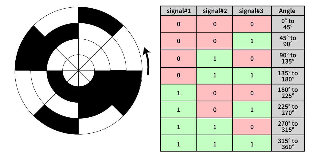
With 3 subdivisions, you can divide the circle in
Commonly, you'll see encoders with one of the following resolutions.
| a | b | c | |
| 1 | Resolution (bits) | divisions | Resolution (degrees) |
|---|---|---|---|
| 2 | 8 | 256 | 1.40 |
| 3 | 10 | 1024 | 0.35 |
| 4 | 11 | 2048 | 0.17 |
| 5 | 12 | 4096 | .09 |
Reading Absolute Encoders
The typical encoder we use in FRC is the Rev Through Bore Encoder . This is a 10 bit encoder, and provides interfaces by either
- Plugging it into the Spark Max
- Plugging it into the RoboRio's DIO port.
Connected as a RoboRio DIO device
When plugged into the RoboRio, you can interface with it using the DutyCycleEncoder class and associated features.
public class ExampleSubsystem{
	// Initializes a duty cycle encoder on DIO pins 0
	// Configure it to to return a value of 4 for a full rotation,
	// with the encoder reporting 0 half way through rotation (2 out of 4)
	DutyCycleEncoder encoder = new DutyCycleEncoder(0, 4.0, 2.0);

	//... other subsystem code will be here ...

	public void periodic(){
		//Read the encoder and print out the value
		System.out.println(encoder.get());
	}
}
Real systems will likely use encoder ranges of 2*Math.PI (for Radians) or 360 (for degrees).
The "zero" value will depend on your exact system, but should be the encoder reading when your system is at a physical "zero" value. In most cases, you'd want to correlate "physical zero" with an arm horizontal, which simplifies visualizing the system, and calculations for FeedForwards for Arm subsystems later. However, use whatever makes sense for your subsystem, as defined by your Robot Design Analysis's coordinate system.
Connected as a Spark Max device
When a Through Bore Encoder is connected to a Spark, it'll look very similar to connecting a Relative Encoder in terms of setting up the Spark and applying/getting config, with a few new options
ExampleSubsystem extends SubsystemBase{
	SparkMax motor = new SparkMax(10, MotorType.kBrushless);
	// ... other stuff
	public void ExampleSubsystem(){
		SparkBaseConfig config = new SparkMaxConfig();

		//Configure the reported units for one full rotation.
		// The default factor is 1, measuring fractions of a rotation.
		// Generally, this will be 360 for degrees, or 2*Math.PI for radians
		var absConversionFactor=360;
		config.absoluteEncoder
		.positionConversionFactor(absConversionFactor);
		//The velocity defaults to units/minute ; Units per second tends to
		//preferable for FRC time scales.
		config.absoluteEncoder
		.velocityConversionFactor(absConversionFactor / 60.0);
		//Configure the "sensor phase"; If a positive motor output
		//causes a decrease in sensor output, then we want to set the
		// sensor as "inverted", and would change this to true.
		config.absoluteEncoder
		.inverted(false);

		motor.configure(
			config,
			ResetMode.kResetSafeParameters,
			PersistMode.kPersistParameters
		);
	}
	// ... other stuff
	public void periodic(){
		//And, query the encoder for position.
		var angle = motor.getAbsoluteEncoder().getPosition();
		var velocity = motor.getAbsoluteEncoder.getVelocity();
		// ... now use the values for something.
	}
}
Discontinuities
Remember that the intent of an absolute encoder is to capture your system state directly. But what happens when your system can exceed the encoder's ability to track it?
If you answered "depends on the way you track things", you're correct. By their nature absolute encoders have a "discontinuity"; Some angle at which they jump from one end of their valid range to another. Instead of [3,2,1,-1,-2] you get [3,2,1,359,358]! You can easily imagine how this messes with anything relying on those numbers..
For a Through Bore + Spark configuration, by default it measures "one rotation", and the discontinuity matches the range of 0..1 rotations , or 0..360 degrees with a typical conversion factor. This convention means that it will not return negative values when read through motor.getAbsoluteEncoder().getPosition() !

Unfortunately, this convention often puts the discontinuity directly in range of motion, meaning we have to deal with it frequently. PID controllers especially do not like discontinuities in their normal range.
Ideally, we can move the discontinuity somewhere we don't cross it due to physical hardware constraints.
There's a few approaches you can use to resolve this, depending on exactly how your system should work, and what it's built to do!
Zero Centering
This is the easiest and probably ideal solution for many systems. The Spark has a method that changes the system from reporting [0..1)rotations to (-0.5..0.5]. rotations. Or, with a typical conversion factor applied, (-180..180] degrees.
ExampleSubsystem extends SubsystemBase{
	// ... other stuff
	public void ExampleSubsystem(){
		SparkBaseConfig config = new SparkMaxConfig();
		config.absoluteEncoder.zeroCentered(true);
		// .. other stuff
		}
	}
Most FRC systems won't have a range of 180 degrees, making this a very quick and easy fix.
Rev documentation makes it unclear if zeroCentered(true) works as expected with the onboard Spark PID controller.
If you test this, report back so we can replace this warning with correct information.
Handle the Discontinuity in your Closed Loop
Since this is common, some PID or Closed Loop controllers can simply take the discontinuity directly in their configuration. This bypasses the need to fix it on the sensor side.
For Sparks, the configuration option is as follows:
sparkConfig.closedLoop.positionWrappingInputRange(min,max);
Be mindful of how setpoints are wrapped when passed to the controller! Just because the sensor is wrapped, doesn't mean it also handles setpoint values too.
If the PID is given an unreachable setpoint due to sensor wrapping, it can generate uncontrolled motion. Make sure you check and use wrapper functions for setpoints as needed.
Handle the discontinuity in a function
In some cases, you can just avoid directly calling motor.getAbsoluteEncoder().getPosition(), and instead go through a function to handle the discontinuity. This usually looks like this
// In a subsystem using an absolute encoder
private double getAngleAbsolute(){
	double absoluteAngle = motor.getAbsoluteEncoder().getPosition();
	// Mote the discontinuity from 0 to -90
	if(absoluteAngle>270){
		absoluteAngle-=360;
	}
	return absoluteAngle;
}
This example gives us a range of -90 to 270, representing a system that could rotate anywhere but straight downward.
This pattern works well for code aspects that live on the Roborio, but note this doesn't handle things like the onboard Spark PID controllers! Those still live with the discontinuity, and would cause problems.
Transfer the reading to a relative encoder
Instead of using the Absolute encoder as it's own source of angles, we simply refer to the Relative Encoder. In this case, both encoders should be configured to provide the same measured unit (radians/degrees/rotations of the system), and then you can simply read the value of the absolute, and set the state of the relative.
More information for this technique is provided at Homing Sequences, alongside other considerations for transferring data between sensors like this.
Build Teams, Code, and Encoders
Since an absolute encoder represents a physical system state, an important consideration is preserving the physical link between system state and the sensor.
On the Rev Through Bore, the link between system state and encoder state is maintained by the physical housing, and the white plastic ring that connects to a hex shaft.
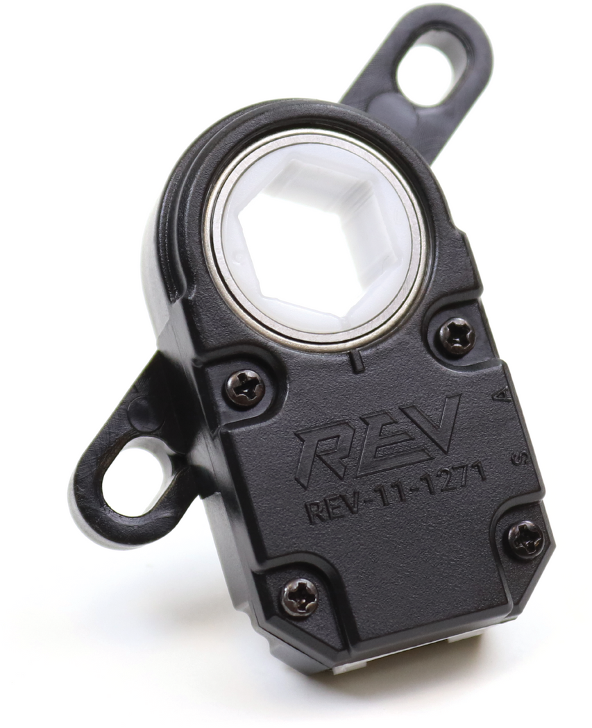
You can see that the white hex ring has a small notch to help track physical alignment, as does the black housing. The notch's placement itself is unimportant; However, keeping the notch consistency aligned is very important!
If we take a calibrated, working system, but then re-assemble it it incorrectly, we completely skew our system's concept of what the physical system looks like. Let's take a look at an example arm.

We can see in this case we have a one-notch error, which is 60 degrees. This means that the system thinks the arm is pointing up, but the arm is actually still rather low. This is generally referred to as a "clocking" error.
When we feed an error like this into motor control tools like a PID, the discrepancy means the system will be driving the arm well outside your expected ranges! This can result in significant damage if it catches you by surprise.
As a result, it's worth taking the time and effort to annotate the expected alignment for the white ring and the other parts of the system. This allows you to quickly validate the system in case of rework or disassembly.
Ideally, build teams should be aware of the notch alignment and it's impact! While you can easily adjust offsets in code, such offsets have to ripple through all active code branches and multiple users, which can generate a to a fair amount of disruption. However, in some cases the code disruption is still easier to resolve than further disassembling and re-assembling parts of the robot. It's something that's bound to happen at some point in the season.
Further Reading
Grey Code
Grey code encoders use binary subdivision similar to the "binary encoder" indicated above, but structure their divisions and output table differently. These differences make for some useful properties:
- Only one bit changes at a time during rotation
- Subdivisions are grouped in a way that reduces the rate of change on any given track
If you look closely, the Quadrature signal used by Relative Encoders is a special case of a 2 bit Grey Code! Looking for this "quadrature" pattern where each track has a 50% overlap to the change across adjacent tracks is a giveaway that an encoder is using gray code.
Analog absolute Encoders
In certain systems, you can measure an X and a Y offset, generating a sin and cosine value. The unique sin and cos values generate a unique angle with high precision.
Fun Theory: Range extension through gearing
In some cases like an Elevator you might want to track motion across a larger range than a single encoder could manage. This is most common for linear systems like Elevators.
By stepping an encoder down, can convert 1 rotation of travel (maybe ~1-3 inches at ~0.01" precision) into a more useful ~50 inches at ~0.5" precision! This gives you absolute knowledge of your system, but at a much lower precision.
However, if you were to stack a normal encoder on top, you could use each encoder within their optimal ranges: One encoder can provide a rough area, and the other can provide the precision.
Fun Theory: Chinese Remainder Theorem
This is a numerical trick that can allow use of two smaller encoders and some clever math to extend two encoders ranges out a significant distance at high precision. This would permit absolute encoders to effectively handle Elevator systems or other linear travel.
TODO
- Advantages
- Disadvantages
- Discontinuity handling
- Integration with relative encoders
Homing Sequences
Git Basics
Goals
Understand the typical Git operations most helpful for day-to-day programming
Completion Requirements
This module is intended to be completed alongside other tasks: Learning Git is best done by doing, and doing requires having code to commit.
- Read through the Git Fundamentals section
- Initialize a git repository in your project
- Create an initial commit
- Create several commits representing simple milestones in your project
- When moving to a new skill card, create a new branch to represent it. Create as many commits on the new branch as necessary to track your work for this card.
- When working on a skill card that does not rely on the previous branch, switch to your
mainbranch, and create a new branch to represent that card. - On completion of that card (or card sequence), merge the results of both branches back into Main.
- Upon resolving the merge, ensure both features work as intended.
Topic Summary
- Understanding git
- workspace, staging, remotes
- fetching
- Branches + commits
- Pushing and pulling
- Switching branches
- Merging
- Merge conflicts and resolution
- Terminals vs integrated UI tools
Git Fundamentals
Git is a "source control" tool intended to help you manage source code and other text data.
Git has a lot of utility, but the core concept is that git allows you to easily capture your files at a specific point in time. This allows you to see how your code changes over time, do some time travel to see how it used to look, or just see what stuff you've added since your last snapshot.
Git does this by specifically managing the changes to your code, known as "commits". These build on each other, forming a chain from the start of project to the current code.
At the simplest, your project's history something like the following
Git is very powerful and flexible, but don't be intimidated! The most valuable parts of git are hidden behind just a few simple commands, and the complicated parts you'll rarely run into. Bug understanding how it works in concept lets you leverage it's value better.
Diffs
Fundamental to Git is the concept of a "difference", or a diff for short. Rather than just duplicating your entire project each time you want to make a commit snapshot, Git actually just keeps track of only what you've changed.
In a simplified view, updating this simple subsystem
/**Example class that does a thing*/
class ExampleSubsystem extends SubsystemBase{
	private SparkMax motor = new SparkMax(1);
	ExampleSubsystem(){}
	public void runMotor(){
		motor.run(1);
	}
	public void stop(){/*bat country*/}
	public void go(){/*fish*/}
	public void reverse(){/*shows uno card*/}
}
to this
/**Example class that does a thing*/
class ExampleSubsystem extends SubsystemBase{
	private SparkMax motor = new SparkMax(1);
	private Encoder encoder = new Encoder();
	ExampleSubsystem(){}
	public void runMotor(double power){
		motor.run(power);
	}
	public void stop(){/*bat country*/}
	public void go(){/*fish*/}
	public void reverse(){/*shows uno card*/}
}
would be stored in Git as
class ExampleSubsystem extends SubsystemBase{
	private SparkMax motor = new SparkMax(1);
+	private Encoder encoder = new Encoder();
	ExampleSubsystem(){}
-	public void runMotor(1){
-		motor.run(1);
+	public void runMotor(double power){
+		motor.run(power);
	}
	public void stop(){/*bat country*/}
With this difference, the changes we made are a bit more obvious. We can see precisely what we changed, and where we changed it.
We also see that some stuff is missing in our diff: the first comment is gone, and we don't see go(), reverse() or our closing brace. Those didn't change, so we don't need them in the commit.
However, there are some unchanged lines, near the changed lines. Git refers to these as "context". These help Git figure out what to do in some complex operations later. It's also helpful for us humans just taking a casual peek at things. As the name implies, it helps you figure out the context of that change.
We also see something interesting: When we "change" a line, Git actually
- Marks it as deleted
- adds a new line that's almost the same
Simply put, just removing a line and then adding the new one is just easier most of the time. However, some tools detect this, and will bold or highlight the specific bits of the line that changed.
When dealing with whole files, it's basically the same! The "change" is the addition of the file contents, or a line-by-line deletion of them!
Commits + Branches
Now that we have some changes in place, we want to "Commit" that change to Git, adding it to our project's history.
A commit in git is a just a collection of smaller changes, along with some extra data for keeping track. The most relevant is
- A commit "hash", which is a unique key representing that specific change set
- The "parent" commit, which these changes are based on
- The actual changes + files they belong to.
- Date, time, and author information
- A short human readable "description" of the commit.
These commits form a sequence, building on top from the earliest state of the project. We generally assign a name to these sequences, called "branches".
A typical project starts on the "main" branch, after a few commits, you'll end up with a nice, simple history like this.
It's worth noting that a branch really is just a name that points to a commit, and is mostly a helpful book-keeping feature. The commits and commit chain do all the heavy lifting. Basically anything you can do with a branch can be done with a commit's hash instead if you need to!
Multiple Branches + Switching
We're now starting to get into Git's superpowers. You're not limited to just one branch. You can create new branches, switch to them, and then commit, to create commit chains that look like this:
Here we can see that mess for qual 4 and mess for qual 8 are built off the main branch, but kept as part of the competition branch. This means our main branch is untouched. We can now switch back and forth using git switch main and git switch competition to access the different states of our codebase.
We can, in fact, even continue working on main adding commits like normal.
Being able to have multiple branches like this is a foundational part of how Git's utility, and a key detail of it's collaborative model. This is more traditionally referred to as a "git tree", since we can see it starts from a single trunk and then branches out into all these other branches.
However, you might notice the problem: We currently can access the changes in competition or main, but not both at once.
Merging
Merging is what allows us to do that. It's helpful to think of merging the commits+changes from another branch into your current branch.
If we merge competition into main, we get this. Both changes ready to go! Now main can access the competition branch's changes.
However, we can equally do main into competition, granting competition access to the changes from main.
Now that merging is a tool, we have unlocked the true power of git. Any set of changes is built on top of each other, and we can grab changes without interrupting our existing code and any other changes we've been making!
This feature powers git's collaborative nature: You can pull in changes made by other people just as easily as you can your own. They just have to have the same parent somewhere up the chain so git can figure out how to step through the sequence of changes.
Workspace, Staging, and Commits
When managing changes, there's a couple places where they actually live.
The most apparent one is your actual code visible on your computer, forming the "Workspace". As far as you're concerned, this is just the files in the directory, or as seen by VSCode. However, Git sees them as the end result of all changes committed in the current branch, plus any additional, uncommitted changes.
The next one is "staging": This is just the next commit, but in an incomplete state. When setting up a commit, staging is where things are held in the meantime. Once you complete a commit, the staging area is cleared, and the changes are moved to a proper commit in your git tree.
Staging is not quite a commit, as the changes represented here can be easily over-written by staging new changes from your Workspace. But, it's not quite the workspace either, and doesn't automatically follow modifications to your code.
Because of this, Staging is extremely useful for code review! Staging a specific change is a great way to assert that that part is working and tested, even if you're not ready to make a commit yet.
In terms of our usual git tree, Staging and Workspace fit in right at the end, like so.
Lastly, is the actual commits that form your history. We generally won't deal with them individually, and instead just bundle them up in "branch". A branch is is just a helpful shorthand that names a specific commit, but in practice is used to refer to all prior changes leading up to that current commit.
Remotes + Github
Git is a distributed system, and intentionally designed so that code can be split up and live in a lot of different places at once, but interact with each other in sensible ways for managing the code.
The most obvious place it lives is your computer. You have a full copy of the git tree, plus your own staging and workspace. This is often called the "local" repository.
Next is a "remote" repository, representing a remote git server. Often this is Github, using the default remote name of "origin".
The important consideration is that your computer operates totally independently of the remote unless you intend to interact with it! This means you can do almost any Git task offline, and don't even need a remote to make use of Git.
Of course, being set up this way means that if you're not paying attention, you might not catch differences between Remote and Local git states. It's rarely an actual problem, but can be confusing and result in extra work. It's good practice to be aware of where your code is relative to origin, and make sure you push your code up to it when appropriate.
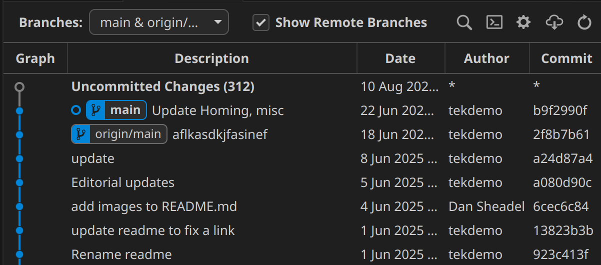
When the origin is indicated specifically, you'll see it shown before the branch name: Main would go from main -> origin/main, like you see here in Git Graph, showing that we have 1 commit locally that doesn't exist on the origin. Or, we're ahead by one commit.
Handling Merge Conflicts
Often when doing merges, you'll run into a "merge conflict", and some parts of your code get replaced with massive compiler errors and weird syntax. Don't panic!
Merge conflicts happen when two branches change the same code. Git can't figure out what the "right answer" is, and so it needs a helping hand. To facilitate this, it has some special syntax so that you can see all information at a glance, but it's not always obvious that it's just being helpful!
Let's look at the simplest possible merge conflict: Being in main, and merging dessert
From an original file containing
Best food is pizza
The commit in main has the following change
-Best food is pizza
+Best food is salad
with dessert having this change
-Best food is pizza
+Best food is cheesecake
The merge is then making Git decide what's the optimal food. Git is not equipped for this debate, so it's up to us humans. Git prepares the file in question using "merge markers" around the issue, which provide some useful info to resolve it
<<<<<<< HEAD
Best food is salad
=======
Best food is cheesecake
>>>>>>> dessert
<<<<<<< HEAD -> indicates the start of a merge conflict. HEAD just means "last commit on current branch". Since we're on main, that means this code is just the result of following the code along the Main branch. VSCode will add additional information above this to help clarify.
>>>>>>> dessert -> is the end of merge conflict. dessert is the branch you're merging from; In other words, it's the result of following the proposed changes along the cheesecake branch. Again, VSCode will add additional info to help.
======= -> is the separator between the two branches' code.
It's helpful to remember the goal of a merge: To put the two codebases together in a way that makes sense and is correct! So a merge conflict is resolved by making code that works, meaning there's several different ways to fix it!
One option is just accepting the change in your current branch, yielding
Best food is salad
This just means you've ignored the proposed change from the other branch (dessert in this case)
The other option is accept the incoming change, and ignore what your branch had.
Best food is cheesecake
In some cases it's both! Maybe you're just fine with two best foods.
Best food is salad
Best food is cheesecake
Of course, you're after correctness. It's possible that after the update neither branch is quite right, and you have to adjust both.
Best side dish is salad
Best dessert is cheesecake
Or, it could be neither! Maybe the right solution has become something else entirely.
Best food is breakfast burritos
Most of the time, a merge conflict should be very easy to deal with if you know the parts of the code you're working with.
Just move the code around until it works like both branches expected, then delete the merge marker, separator, and any unnecessary code, and you're good to go!
And, don't worry if you missed one! Git will spot these conflict markers if you try to commit one without sorting it out.
If you get lost, ask for help! When dealing with code someone else wrote, you simply might not know what the best option is when coming out of it. That's fine! No tool can replace good communication.
Handling Compile errors caused by merges
Merge conflicts aside, just because a merge didn't have a conflict, doesn't mean the code works. A sometimes surprising result stems from the fact that Git doesn't understand code, it just understands changes!
The most likely reason you'll see this is someone changing a function name in one branch, while the other branch adds a new occurrence of it. Let's consider adding this code in our current branch
@@ MainBranch: RobotContainer.java @@
   //filecontext
+  exampleSubsystem.callSomeFunction();
   //filecontext
and merging in this change from another branch.
@@ CleanupBranch: ExampleSubsystem.java @@
   //filecontext
-  public void callSomeFunction(){
+  public void betterNamedFunction(){
   //filecontext
In this case, main doesn't know about the name change, and CleanupBranch doesn't know that you added a new call to it. This means callSomeFunction() no longer exists, leading to an error.
As with merge conflicts, it's up to you to figure out what's correct. In cases like this, you just want to adjust your new code to use the new name. But it sometimes happens that the other branch did something that needs to be changed back, such as deleting a function no one was using... until now you're using it.
Again, the purpose of the merge is to make it work! You're not done with a merge until everything works together as intended.
The critical Git commands
A lot of Git's power boils down to just using the simple usage of a few basic commands.
While using the command line is optional, most good Git tools retain the name of these operations in graphical interfaces. After all, they're using the same operations behind the scenes.
Because of this, a bit of command line knowledge can help clarify what the more user-friendly tools are trying to do, and show you exactly why they're helpful.
Creating a new repository
git init will creates a new git repository for your current project. It sets the "project root" as the current folder, so you'll want to double-check to make sure you're in the right spot!
VSCode's built in terminal will default to the right folder, so generally if your code compiles, you should be in the right spot. Once the repository is created, git commands will work just fine from anywhere inside your project.
Getting Status
Knowing what your code is up to is step 1 of git. These commands
git status just prints out the current repo status, highlighting what files are staged, and what have unstaged changes, and where you are relative to your remote. If you've used other git commands, the effects will show up in git status. Run it all the time!
git log will open a small terminal dialogue walking you through changes in your branch (hit q to exit). However, it's often unhelpful; It contains a lot of data you don't care about, and is missing clarity on ones you do.
git log --oneline tends to be more helpful ; This just prints a one-line version of relevant commits, making it much more useful.
Adding Changes to build a commit
git add <files> is all that's needed in most cases: This will add all changes present in a specific file.
git add <directories> works too! This adds all changes below the specified folder path. Be mindful to not add stuff you don't want to commit though! Depending on the project and setup, you may or may not want to add all files this way.
git add . is a special case you'll often see in git documentation; . is just a shorthand for "the current folder" . Most documentation uses this to indicate "Stage the entire project", and is mostly helpful for your very first commit. Afterwards, we'd recommend a more careful workflow.
git reset <staged file/dir> will will remove a file's changes from Staging and put them back in the Workspace ; Meaning, the change itself is preserved, but it won't be changed. In practice, you probably won't do this much, as it's easier to use a GUI for this.
Confirming a commit
git commit -m "describe changes here" tends to be the beginner friendly approach. This makes a new commit with any staged changes.
git commit will usually open a small terminal editor called Vim with commit information and let you type a commit message. However, this editor is famous for it's "modal" interface, which is often surprising to work with at first. We'll generally avoid using it in favor of VSCode's commit tooling.
If you get caught using the Vim editor for a commit, this is a quick rundown of the critical interaction.
escape key-> undo whatever command you're doing, and and exit any modes. Mash if you're panicking.
i -> When not in any mode, enter Insert mode (INSERT will be shown at the bottom). You can then type normally. Hit escape to go back to "command mode"
: -> start a command string; Letters following it are part of an editor command.
:w -> Run a write command (this saves your document)
:q -> Run a quit command (exit the file). This will throw an error if you have unsaved changes.
:q! -> The ! will tell Vim to just ignore warnings and leave. This is also the "panic quit" option.
:wq -> Runs "save" and then "quit" using a single command
This means the typical interaction is i (to enter insert mode), type the message, escape, then :wq to save and quit.
You can also abandon a commit by escape + :q!, since an empty commit message is not allowed by default.
Creating Branches
git branch NameOfNewBranch: This just makes a new branch with the current name. Note, it does not switch to it! You'd want to do that before trying to do any commits!
Note, the parent node is the last commit of your current branch; This is not usually surprising if you're working solo, but for group projects you probably want to make sure your local branch is up to date with the remote!
Switching Branches
git switch NameOfBranch: This one's pretty simple! It switches to the target branch.
git switch --detach <commithash> : This lets you see the code at a particular point in time. Sometimes this can be useful for diagnosing issues, or if you want to change where you're starting a new branch (maybe right before a merge or something). --detach just means you're not at the most recent commit of a branch.
You might see git checkout NameOfBranch in some documentation; This is a common convention to "check out" a branch. However, the git checkout command can do a lot of other stuff too. For what we need, git switch tends to be less error prone.
Note, Git will sometimes block you from changing branches! This happens if you have uncommitted changes that will conflict with the changes in the new branch. It's a special kind of merge conflict.
Git has a number of tools to work around this, but generally, there's a few simpler options, depending on the code in question
- Delete/undo the changes: This is a good option if the changes are inconsequential such as accidental whitespace changes, temporarily commented out code for testing, or "junk" changes. Just tidy up and get rid of stuff that shouldn't be there.
- Clean up and commit the changes: This is ideal if the changes belong to the current branch, and you just forgot them previously
- "Work in progress" commit: If you can't delete something, and it's not ready for a proper commit, just create a commit with message beginning with "WIP"; This way, it's clear to you and others that the work wasn't done, and to not use this code.
- use "git stash" the changes: This is git's "proper" resolution for this, but the workflow can be complicated, easy to mess up, and it's out of scope for this document. We won't use it often.
Merging code
git merge otherBranchName : This grabs the commits from another branch, and starts applying them to your current branch. Think of it as merging those changes into yours. If successful, it creates a merge commit for you.
git merge otherBranchName --no-commit : This does the merge, but doesn't automatically make a commit even when successful! This is often preferable, and makes checking and cleanup a bit easier. Once you've ran it, you can finish the commit in the usual way with git commit
git merge --abort is a useful tool too! If your merge is going wrong for whatever reason, this puts you back to where you were before running it!
git merge (note no branch name) merges in new commits on the same branch; This is useful for collaborate projects, where someone else might update a branch.
Keeping up to date with a Remote
git fetch connects to your remote (Github), and makes a local copy of everything the remote system has! This is one of the few commands that actually needs internet to function.
Note, this does not change anything on your system. It does as the name implies, and just fetches it. Your local copies of branches remain at the commit you left them, so git fetch is always safe to run, and some tools run it automatically.
Pulling code from a remote + updating branches
git pull will contact the remote system, and apply changes from the remote branch to your local branch.
Behind the scenes, this is just running git fetch and then git merge. So, if you run git fetch and then try to work without internet, you can still get things done! Just use git merge with no branch name.
Pushing code to a remote
git push does this. By default it uses the same name, making this a short and simple one.
git push will fail if the push would cause a merge conflict on the remote system. This can happen if the remote branch has been modified since you branched off of it.
If this happens, you'll need to update your repository with git fetch or git pull , resolve the conflict, and try again
Git from VSCode
Handling Git operations from VS Code is normally a very streamlined operation, and it has good interfaces to do otherwise tricky operations.
Git Graph Plugin
This plugin provides some notable visualization tools that further improves Git handling in VS Code. We'll assume this is installed for the remainder of the tutorial here.
https://marketplace.visualstudio.com/items?itemName=mhutchie.git-graph
Install that first!
Git Sidebar
The icon on left side will open the git sidebar, which is the starting point for many git operations.
Opening it will provide some at a glance stuff to review.
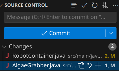
We can see a lot of useful things:
At the top we can see any uncommitted changes, and the file they belong to. We'll deal with this when reviewing changes and making new commits.
At the bottom (which might be folded down and labelled > Outline or > Graph), we can see our commit history for the current branch. The @main represents the current branch state, and icon represents the Origin (Github). If we're ahead or behind the origin, we can see it at a glance here.
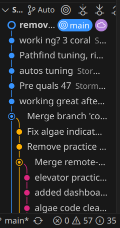
Note, we also see main at the very bottom; That's always there, giving us our current branch at a glance.
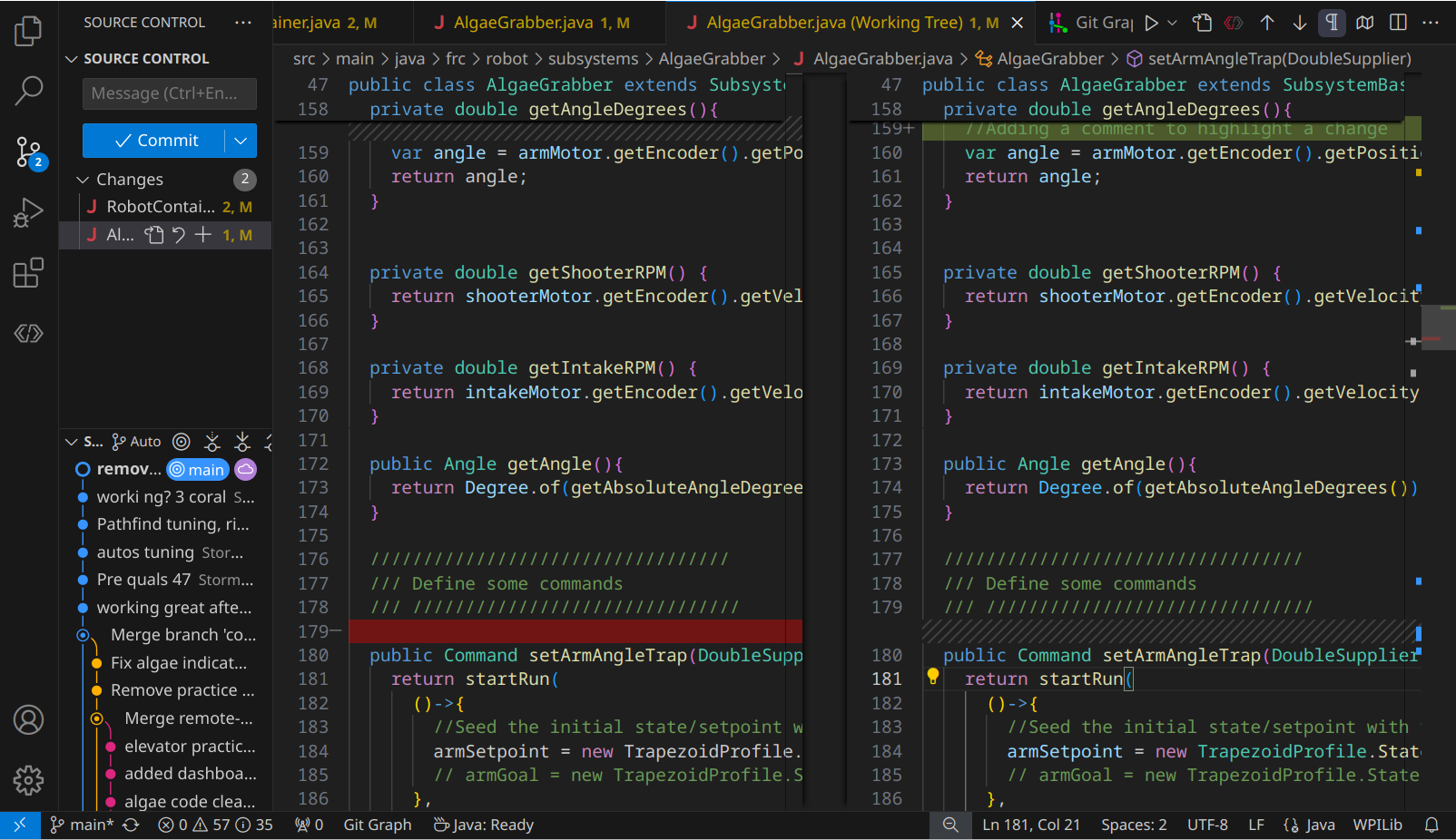
Reviewing Changes + Making commits
The easiest way to review changes is through the Git Sidebar: Just click the file,and you'll see a split view.
Changes will be shown in one of two ways. "Additions" are shown as a green highlight on the right side. On the left, you can see a ///////////////// placeholder; This helps align the code so that you can easily keep track of where stuff gets inserted!
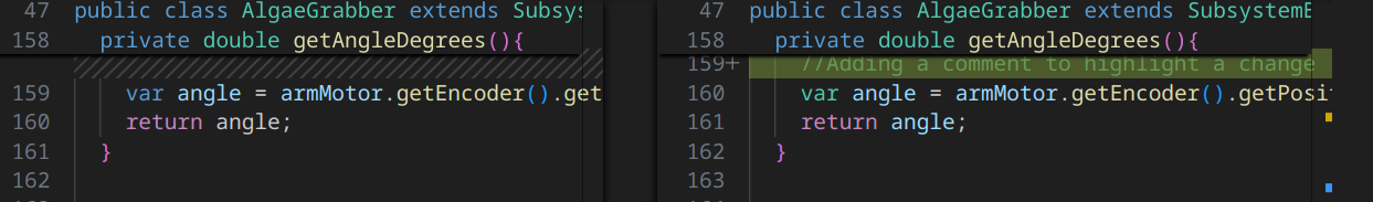
Deletions look similar, but reversed. Left gets a red, right gets a placeholder.
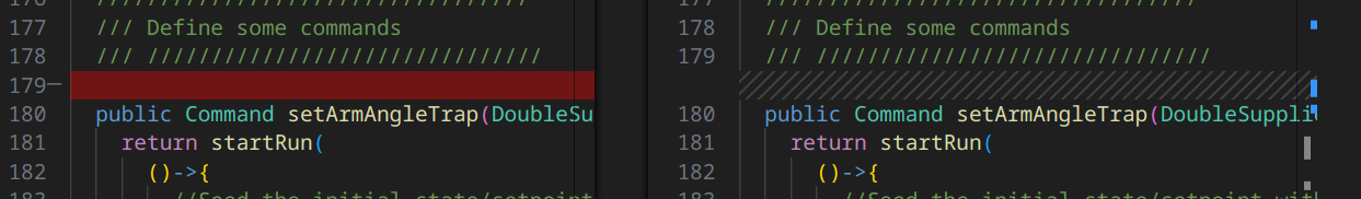
Changes to part of a line are either an addition and removal, or a small highlighted change of the particular bits.
Note, you can actually type here! The right hand side is editable, allowing you to revise things if you see a change that's concerning. That side just represents the current state of the file in the workspace.
The left side is locked; This represents the prior state of the file, which can only be changed by adding more commits.
You can approve/confirm changes in a couple ways. The easiest is to simply use the "Stage Changes" button by the filename in the sidebar; This stages all changes in a particular file.
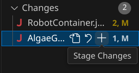
In many cases, it's helpful to handle them one by one: If you right click on a change (or selected text that includes one or more changes), you'll see some options besides the normal text editing ones
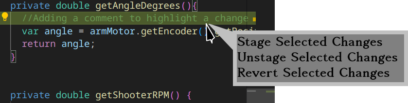
As the name implies, you can Stage changes if you want them, Unstage them (if you want to remove it from the commit you're putting together).
Note, you can also Revert it. In this case, reverting means that the change is gone! Added lines vanish, changed numbers go back to what they were, and reverting a deletion puts all the lines back! Be very careful here to not undo your work!
Note, that there's also a Revert/Discard Changes button too! Fortunately, this one checks with you. We'll rarely use it, but make sure to not hit it accidentally!
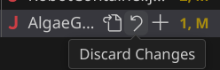
Once we've staged some changes, we'll any staged changes separate from any unstaged changes
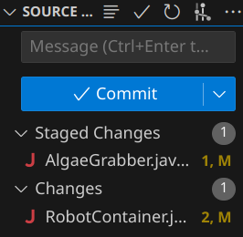
You can commit with un-staged changes just fine, just be mindful! We'll touch on best practices later.
Once you've added all changes you want to include in the commit, just enter the message and click "Commit". Done!
Remote interactions + VS Code
VS Code has some useful built in operations to push or pull branches! These will typically pop up automatically, with the helpful options being
Push-> Does a standard pushPull-> Does a standard pullPublish Branch-> This is a normal Push, but applies to newly created local branches. This normally requires a couple other small steps, which this handles automaticallySync-> Don't use this one!
Be careful about the "Sync" button! Unlike other VSCode options, "Sync" will try to push and pull at the same time; However, in case of a merge conflict, it might try to resolve it using esoteric git operations behind the scenes. While this sometimes works, when something goes wrong fixing it properly is extremely challenging!
In almost all cases, using a git pull , verifying the merge, and then a git push is a better workflow!
Viewing the git tree with Git Graph
We're now looking at the Git Graph specific stuff, so make sure that's installed!
There's two ways to launch it. One is using VS Code's Command Palette, activated by CTRL+Shift+P then typing "View Git Graph" or "git log" to pull up this particular one.
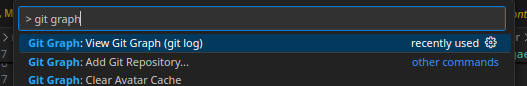
The other is by clicking "Git Graph" along the bottom toolbar.
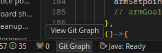
Both of these will take you to a good review interface, where you can see the status of many branches, the commit log, and how things merged and diverted! This is from our 2025 season code.
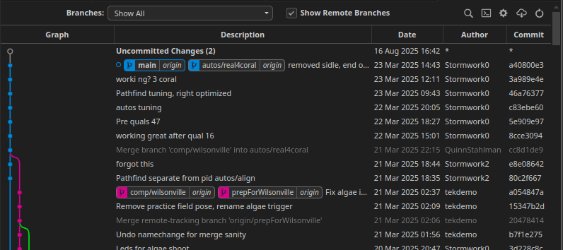
Just this interface provides a lot of value: You can easily see the commit history, how branches have diverged and been merged, and check to see what branches are ahead or behind of the origin.
If you click a commit, you get a more detailed status, but most notably what files were altered.
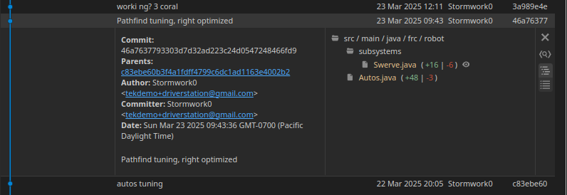
And, if you click the file in the commit details, it'll show you what that commit changed!
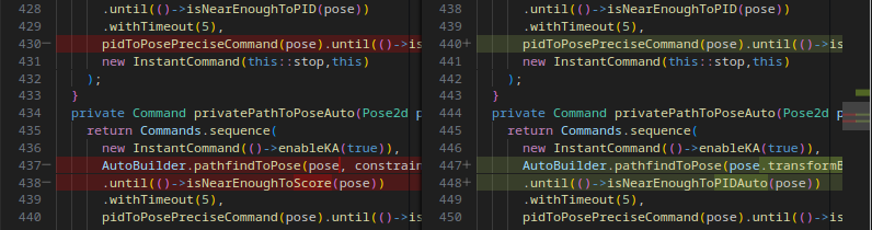
This is a very fast and effective way to look through your project and catch up on what's happening.
There's a lot of other value here if you click around, including being able to right click and checkout or switch to various branches!
VSCode's Git Terminal
VS Code's terminal often pops up during many other operations, but if you don't see it, you can access it through the menu.
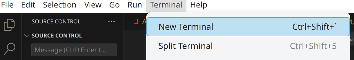
Since we usually work on Windows, this will often open up a Powershell, which is usually sub-optimal for what we want to use a terminal for. Git Bash is usually nicer. You can change this with the Command Pallete (CTRL+Shift+P), and selecting Terminal: Select Default Profile.
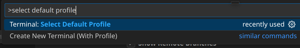
If Bash is available, click it! Any new terminals will use the Git bash, which will have color, some at-a-glance git info, and generally more helpful all around.
Other Git tools
There's a lot of tools that interact with your Git repository, but it's worth being mindful about which ones you pick! A lot of tools wind up changing normal git operations into renamed or altered versions that do a lot of things at once. This can make learning it harder, and if something goes wrong, fixing the results can be extremely difficult. Stick to the basics until you know what's happening and you can properly judge if a new tool is worth using.
Making the best use of git in FRC
A typical FRC workflow
Creating the initial project setup:
git initto set up our new project.git add .to stage all the files in their blank, default state- Commit the code, using VSCode's interface or with the terminal
git commit -m "initial commit"
Doing the code work:
git branch featurebeingaddedto set up a new branch for your taskgit switch featurebeingaddedto select your new branch- Add the code
- Review the new code using VSCode, staging parts that are confirmed to work
- Commit the code (via Code or terminal)
- Repeat commits until done
Handling review and merging. Be mindful of local and remote branch states for this!
- Test and review your code! Make sure it works in the final state.
git fetchto ensure your git repo is aware of any changes.git merge origin/main --no-commit-> Bring in all new changes- Fix, test, review your code with all the new base project code.
git committo finalize the merge.git pushto push your branch with the merge completed.- Work with your maintainer (a mentor or veteran) to pull your new, validated changes back into
main!
Feature Branches
Branches are best when they're small, focused, and well defined.
A great workflow is using so called "topic branches" or "feature branches": In this workflow, a branch represents a feature you're adding, or a bug you're fixing. Once the feature is added and working, the branch is Done. You merge your branch back into the Main branch, and you can move onto another feature in a new branch!
By doing this, you keep each branch simple, easy to test, and easy to merge. It also helps prevent the issue of long-running branches; Where your code is isolated from a long time, and drifts apart from everyone else's code in main. That ends up with you not working on quite the same code base as other people, and you'll miss out on features, fixes that everyone else has, and they'll miss out on yours.
A good feature branch name also helps keep you as a programmer constrained to the task at hand.
Branch Naming
To facilitate "feature branch" convention, name your branches after feature itself, rather than the part of code it's affecting. Make sure that the branch name implies an "end state" at which point you can consider it Done and stop working on it.
As an example, some good initial branch names are add-far-shots, add-climb-routine, or fix-intake-stalling-issue. Since we're usually adding or fixing things, we can often omit that in the actual name leaving us with far-shots, climb-routine, intake-stall-issue), but it's helpful to always pretend it's there unless a clearer verb exists (like remove or adjust.
Early on, you might be tempted to name your branches after robot systems, like intake, shooter, or the like. But don't do this! The intake will always exist on the robot, so your branch has no clear end state!
Instead, name it something like intake-bringup. This provides an end-condition: Once the intake is brought up, functioning, and tested, the branch is done, and you can merge it back into main.
In some cases, it's helpful to indicate which part of the robot you're working on though: The optimal method is using subsystemname/feature. This is especially true of features relevant to various subsystems like bringup, which just yields intake/bringup, elevator/bringup, etc.
Merge other branches into yours
Merging is more useful than just sending your changes back to Main. You can use merging to keep up with other features that interact with the code you're working with.
As an example, let's say you're trying to bring up an Indexer system, which interacts with a Intake and a Shooter. During early development, you might see some branches like this
Intake and Shooter aren't done enough to merge back into main, but the indexer can't really be tested because you need to move it through the intake and shooter. But, you also don't want to actually do all that work yourself.
So, just merge the intake/bringup and shooter/bringup branches!
There you go! Now you can continue your work, using the preliminary work from the other branches. As they adjust and fix things, you can merge their code, and they could also merge yours into their branches before finally verifying 2 or 3 of these subsystems work properly.
There's a catch here: The branches in question might not be fully ready for you to pull them! It's always a good idea to talk to whoever's working on that code to make sure that it's in a state that's good to go. Sometimes they'll just need to adjust up one or two things, fix a variable/method name, or other times they might suggest you wait for some bigger cleanup or process fixes.
Merge main->Topic before Topic->main
Similar in concept to the above in some ways! By our process definitions, Main should always be in a good state, meaning you can pull it at any time. So, before declaring your branch Done and getting it in Main, go ahead and pull Main and test things first!
Now you can test the indexer in the full codebase without any risk of accidentally putting a bug in main, and any adjustments are part of the indexer/bringup branch like shown here
At long last, with everything fully integrated, we can finally get our changes back into main, knowing with confidence it works as expected.
SuperStructure Elevator
Requires:
FeedForwards
PID
Reading Resources:
Homing
Success Criteria
- Create an Elevator subsystem
- Set Encoders
- find the encoder range and conversion to have real-world values
- Find the system range, apply soft limits
- Get control
- Determine the system Gravity feed-forward value
- Create a PID controller
- Tune the PID to an acceptable level for control
- Create a default command that holds the system at the current height
- Create a setHeight function that takes a height, and returns a command that runs indefinitely to the target height
- Create a Trigger that indicates if the system is within a suitable tolerance of the commanded height.
- Bind several target positions to a controller
- Create a small auto sequence that moves to multiple positions in sequence.
Synopsis
Elevators are a common linear motion system in FRC, generally used to raise game pieces from the floor to a high scoring objective.
While mechanically straightforward, Elevators wind up generating a notable step up in code and control complexity compared to Roller systems.
Safety first! Elevator hazards
Elevators introduce several areas where you can inadvertently cause damage to the environment and robot. When prototyping and developing them, there's a few important considerations:
- Elevators have a limited range of motion: Carelessly commanding them beyond their physical constraints can damage the robot, the motors, and eject parts at nearby people!
- Elevators and drive belts/ropes generate many pinch points that can snag fingers if the system is moved by hand, even when disabled.
- Rapid motion can de-stabilize a robot that's sitting on a cart or on blocks
When making changes to elevator behaviors and tuning, make sure someone nearby is ready to disable the robot if anything goes wrong.
PIDS + FeedForwards + Motion Profiles
Controlling an elevator requires the use of a PID, and greatly benefits from aspects of both FeedForwards and Motion Profiles.
A PID by itself can control an elevator, but it will be difficult to tune and require significant time and resources to "hack" into a usable state. Any time you change setpoints, the whole system is in for a bad time: The output power rapidly changes to move to the new position, putting significant strain on the robot, causing excess wear, and potential damage. Moving a significant distance can also slam the elevator carriage into the limits of motion, causing damage.
FeedForwards, or at least the kS and kG terms, will greatly improve stability and accuracy, and reduce the time it takes for tuning a PID. However, it does not mitigate the issues cause changing setpoints.
Motion Profiles fix the setpoint problem, and lock the setpoint changes into a nicely defined ramp-up and ramp-down when changing positions. This means your PID never misbehaves, and provides additional feed-forward information to further simplify tuning.
While the combination may seem daunting at first, each of these 3 solves a particular motion problem effectively, and with straightforward individual adjustments. Using all 3 together provides a better performing system, with much less effort overall.
On occasion, you'll encounter linear systems with extremely high-torque gearing, such as screw-drive systems. These really do perform perfectly fine with just a PID controller, since the motor itself is never loaded, and a full motor output generates a slow motion with little inertia. In that case, you can simply ignore the FeedForward and Motion Profile.
Preparing The Elevator
The first few steps can be done before spinning the motor
- temporarily define the Homing behavior as bootup zero. This streamlines the initial process.
- Calibrate the encoder on the elevator to Inches, and ensure the encoder increases as you gain height. These steps were encountered in Encoder Basics
- Verify the correct calibration and encoder values by moving the elevator by hand when disabled.
- Define soft limits to prevent driving past the frame limits. The important limit is the "reverse" limit heading toward the bottom, but the top limit can be set to an approximate or low value temporarily.
- Estimate and configure a low P value. This will be used for controlled preliminary motion, and just needs to move the system and not oscillate at setpoints.
- Estimate and configure sane maxVelocity and maxAccelleration values for the motion profile.
- plot motor output voltage and height, which you'll need for tuning.
- You will need a
setPowerstyle command that allows arbitrary input.
Tuning
With the system and code prepared, you can now work with the system a bit.
- Determine the approximate system kG: For this, you can use the manual command to drive the motor upward away from the hard stop, then and hold it still. Record the voltage, and add it to your feed-forward.
- Now you can use easily use your manual adjustment command and approximate kG calculate a precise kS and kG, as indicated in FeedForwards > Finding kS and kG. It helps to divide the joystick value by 4 to 10 to give you more range on the physical input side.
- With the FeedForward configured, almost any kP will work to get the system to setpoints, but slowly. If your system is oscillating, you can lower kP.
- Optionally, you can attempt to calculate kV and kA, or use System Identification to assist.
- At this point, your system should be travelling between setpoints fairly cleanly. The plot of your position during motion should be smooth, and your velocity a clean trapezoidal shape.
- Now that you have optimized motion, you can set the upper soft limit properly.
- Check your current limits! Now is a reasonable time to increase them, and you will want to plot them to see what currents are needed so you can limit them properly.
Troubleshooting:
- System oscillates or rattles around setpoint: This is likely due to a high kS value, but it may be caused by a high kP value.
- There's odd hitches/jolts during a motion: Your kV or kA gain is probably too high. Set kA to zero, and then lower kV until it moves smoothly. Then try to add kA back in, lowering if needed. This is possible with a high P gain, but less probable.
- The system drifts up/down: Your kG is too high or too low.
- System not getting to setpoint: If it's not going up enough, kG+kS is too small. If it's not going down enough, kG-kS is too small. Recalculate those two.
- Any of the above, but only when loaded/unloaded with game pieces: This can be caused due to the weight difference causing your gains to no longer properly approximate your system output. One option is to tune for the "lightest" elevator, which should result in stable motion when weight is added, and will lean on the PID to handle the error. The ideal option is to configure two or more feed-forwards, and swap the feed-forward values when each condition occurs.
- Any of the above, but only in some parts of the travel. This can be caused by design quirks, as some elevator configurations have physical differences at different points in travel. Similar to above, you can tune to the "lowest output" variant and let the PID handle problems, or configure several feed-forwards and select them as your elevator enters specific regions of travel.
Optimizing the Motion
If your FF+PID tuning looks good, it's time to play with the Motion Profile. The goal is to make your max Velocity and max Accel as high as possible, representing the fastest possible motion. However, you do not want to set these higher than the system can physically manage, and it should never move so fast as to be unsafe or self-damaging. So, it's something of an iterative, incremental increase until you get the motions you want.
The best two plots for this are
- Current height and setpoint height
- Current velocity and setpoint velocity
These both represent what you're telling the system to do and what it's actually doing.
Once you have plots, you just need two buttons on a controller, moving the elevator to two different heights. You should choose heights far apart to have a relatively long travel, but stays a couple inches away from any hard stops or soft limits. The extra space at the end provides a safety net in case of an error, and allows the system to avoid crashing into them at high speeds. The long travel ensures you can reach high speeds during the motion, and test the max velocity.
Now, you should be able to see both the height and velocity closely track the setpoint versions. There's a few ways that they can deviate
- The velocity setpoint graph is always a triangle, never a trapezoid: This is ok! This just means you're constrained by range and the acceleration. As you increase acceleration, you
- The real velocity/position "lags" behind the setpoint. This is expected if you do not have a kV or kA on your feedforward. Adding a kV will bring them closer together and reduce this lag. A kA can also help, but is less critical.
- The real position/velocity "bounces": See troubleshooting above. It's likely that your P gain is too high.
- Instead of a trapezoidal shape, the velocity start and end have curved lines, and/or overshoots setpoint: This means your max acceleration is too high, and the motor cannot output enough power to hit the target velocity. Check your current limit, increase if needed. If you cannot provide more current, or do not wish to do so, decrease the acceleration until the system is on track.
- The robot emits concerning creaky/crunchy noises: Your acceleration is higher than the bot is capable of surviving. The motor can keep up, but the geartrain will explode in short order. Lower the acceleration until it goes away. Remember, F=M*A : The acceleration is what imparts the force to the elevator.
Homing
Until now, we've assumed an initial physical position against a hard stop. This is perfectly suitable for setup, testing, and diagnostics, but can be hazardous over the full life cycle of a robot.
Every time the battery is changed or the power is cycled, there's a chance that the robot wasn't where you expected, and if caught off guard you can damage the robot pretty severely, on top of failing to play the game as intended.
Elevators tend to require Homing more than other systems, as there's no robust, readily available sensor to capture the height directly.
There's several valid homing strategies, but often elevators start near the lowest point of travel, making it simple to use a Current Detection process. Helpfully, our feed forward analysis also tell you what the needed output power is: something just below
Homing should start automatically (or be run at start of auto), but it's also wise to give Drivers a "home" button just in case. They can't touch the robot on the field, making a home operation a necessary option for recovery from reboots or unexpected field events.
Starter Template With Profiles
This uses the streamlined WPILib ProfiledPIDController providing the simplest complete implementation.
There's many useful methods here : ProfiledPIDController Method Reference
UNITS This is configured to use Volts for feedforward and PID gains, so be mindful!
Homing This template does not include Homing, and assumes a "zeroed on boot" approach. It's recommended to determine and implement a robust strategy for most bots.
ExampleElevator extends SubsystemBase{
	SparkMax motor = new SparkMax(42,MotorType.kBrushless);

	//Define our system's maximum motion constraints
	//When in doubt,
	//- set maxVelocity at a low value. 12 in/s is a great starter value
	//- set kMaxAccelleration high, at roughly 4*kMaxVelocity
	private final TrapezoidProfile.Constraints constraints =
		new TrapezoidProfile.Constraints(kMaxVelocity, kMaxAcceleration);
	//Create a PID that obeys those constraints in it's motion
	//Likely, you will have kI=0 and kD=0
	private final ProfiledPIDController controller =
		new ProfiledPIDController(kP, kI, kD, constraints, 0.02);
	//Our feedforward object
	//When in doubt, set these to zero (equivilent to no feedforward)
	//Will be calculated as part of our tuning.
	private final ElevatorFeedforward feedforward =
		new ElevatorFeedforward(kS, kG, kV);

	ExampleElevator(){
		//These documented below to better demonstrate the general structure
		configMotor();
		configProfiledPID();
		//DefaultCommands help avoid leaving a system in an uncontrolled
		//state. For elevators, we often want no motion
		setDefaultCommand(stop());
		//For systems using an I gain, you likely want to
		//command the PID controller at all times rather than use stop(),
		//which behaves better with the I term's summing behavior.
		//holdPosition() is better than stop() for this use case.
	}

	///Prepare Telemetry for tuning
	public void periodic(){
		var output=motor.getAppliedOutput();
		// We cannot get the applied voltage directly, but since
		// it's a percentage we can multiply by the provided battery voltage
		var voltage=motor.getAppliedOutput()*RobotController.getBatteryVoltage();
		var height=motor.getEncoder().getPosition();
		var velocity=motor.getEncoder().getVelocity();
		var setpoint=controller.getSetpoint();

		SmartDashboard.putNumber("elevator/voltage",voltage);
		SmartDashboard.putNumber("elevator/height",height);
		SmartDashboard.putNumber("elevator/velocity",velocity);
		SmartDashboard.putNumber("elevator/set position",setpoint.position);
		SmartDashboard.putNumber("elevator/set velocity",setpoint.velocity);
	}

	//Triggers form the optimal way to transfer subsystem states/conditions
	//to external subsystems.
	//The PID contains this method, so we can just check it
	//ProfiledPID objects's other useful indicators of completion as well,
	//such as .timeRemaining for the intended motion.
	public Trigger isAtPosition = new Trigger(controller::atGoal);

	/// Return the height of our elevator, using Unit measures
	public Distance getHeight(){
		return Inches.of(motor.getEncoder().getPosition());
	}

	/// Provide manual output. Should only be used for
	/// debugging, tuning, and homing
	public Command setPower(DoubleSupplier percentOutput){
		//Including the feed-forward here, but can be removed
		//if your testing is easier without it.
		return run(()->motor.setVoltage(
			percentOutput.getAsDouble()*RobotController.getBatteryVoltage()
			+ feedforward.getKg()
			)
		);
	}

	/// Disable the elevator's motion entirely
	public Command stop(){
		//Note, an output of 0 usually falls down, which is *not* the
		//same as stopping! So, we instead use kg to resist gravity.
		//A "stopped" subsystem can still be moved by hand or
		//external forces though!
		return setPower(feedforward::getKg)
	}

	///Command the Elevator to go to the target position
	public Command setHeight(Supplier<Distance> position){
		return run(()->{
			//Update our goal with any new targets
			controller.setGoal(position.get().in(Inches));
			//Calculate the voltage contributing to the output
			var vff = feedforward.calculate(controller.getSetpoint().velocity);
			var vpid = controller.calculate(motor.getEncoder().getPosition());
			//Apply to the motor
			motor.setVoltage(vff+vpid);
		});
	}

	/** Set the angle to a fixed value */
	public Command setHeight(Distance position){
		return setAngle(()->position);
	};

	/** Actively maintain the position command was started at */
	public Command holdPosition(){
		//Deferred commands are needed here to capture the angle
		//at the time the command is initiated
		return defer(()->setHeight(getHeight()));
	}

}
// Important configuration parameters for an Elevator subsystem
void configMotor(){
	//These are the important ones for Elevators specifically
	SparkBaseConfig config = new SparkMaxConfig();
	//Default current limit should be low until the system is homed.
	//.. but this requires a homing process.
	config.smartCurrentLimit(40);
	//You want "forward" to be positive, with increasing encoder values
	config.inverted(false);
	//Soft
	config.softLimit
	.forwardSoftLimit(18) //Whatever max height is
	.forwardSoftLimitEnabled(true)
	.reverseSoftLimit(0) //Sometimes zero, or the lost attainable height
	.reverseSoftLimitEnabled(true);
	;
	//The conversion/gearing needed to put your system in a sensible
	// unit; Often Inches.
	var elevatorConversionfactor = 1;
	elevatorConfig.encoder
	.positionConversionFactor(elevatorConversionfactor)
	.velocityConversionFactor(elevatorConversionfactor / 60.0)
	;
	//Apply the configs
	elevatorMotor.configure(
		config,
		ResetMode.kResetSafeParameters,
		PersistMode.kPersistParameters
	);
}

void configProfiledPID(){
	//Configure the ProfiledPIDController

	//This value constraints the output added by the I term
	//in the PID controller. This is very helpful to prevent damage in cases
	//where the elevator system jams or collides with the environment and
	//cannot move.
	// This will be system dependent, and should (needs testing) be
	// in PID ouptut units (normally Volts)
	controller.setIntegratorRange(-1, 1); //Configure to +/-1 volt

	//When the robot is disabled, the elevator might move, invalidating
	// the controller's internal state, and invalidating the I term's sum.
	//This needs to be reset whenever the robot is enabled, and a Trigger
	// provides a clean way of handling this
	new Trigger(DriverStation::isEnabled).onTrue(
		()->controller.reset(motor.getEncoder.getPosition())
	);

	//There's other methods for interacting with the PID values
	// and constraints, should the need arise
}
Advanced usage can easily extend this to handle position dependent constraints, or provide alternate constraints for certain motions.
Using Spark PID control + Elevators
Rev is developing a new Spark API that can run Feedforwards + Motion profiles entirely on the Spark Motor controller.
TrapezoidalProfiles + external PID is messy, and thus documented to a minimal extent below
Implementing mixed Spark PID + Trapezoidal is not strongly recommended, due to the high levels of code jank and surprise complexity, combined with limited benefit in this context. However, a full example can be found in 2025 Stormbots Reefscape
The primary difference from above
- The need to create a Trapazoidal Profile object directly, rather than a ProfiledPID
- You need to set the PID in the trapezoidal Profile to determine the expected state
- Need to query the calculated state and pass the value to the external PID.
- Need to track the "Goal state" for completion testing
Note that a "Goal State" represents the final objective for the trap profile, which is used to calculate setpoints, serving as intermediate targets for motion.
private TrapezpoidProfile.Constraints constraints =
new TrapezpoidProfile.Constraints(
	kElevatorMaxVelocity,
	kElevatorMaxAcceleration
);
private final TrapezoidProfile elevatorTrapezoidProfile =
	new TrapezoidProfile(constraints);

//Needed to store the Final state of the motion so triggers can
//calculate finished motion
TrapezoidProfile.State elevatorGoal=new TrapezoidProfile.State(0,0);
//We also need to retain the intermediate steps; When these match,
//our planned motion has been completed.
TrapezoidProfile.State elevatorSetpoint=new TrapezoidProfile.State(0,0);

private Command setHeight(DoubleSupplier position){
	return new SequentialCommandGroup(
		//Seed the initial state/setpoint with the current state
		//Maybe optional?
		new InstantCommand( ()->{
			elevatorSetpoint = new TrapezoidProfile.State(
				getAngle().in(Degrees),
				elevatorMotor.getEncoder().getVelocity()
			);
		}),

		new RunCommand(()->{
			//Make sure the goal is dynamically updated
			elevatorGoal = new TrapezoidProfile.State(
				position.getAsDouble(),
				0
			);
			//update our existing setpoint to the next achievable state
			elevatorSetpoint = elevatorTrapezoidProfile
				.calculate(0.02, elevatorSetpoint, elevatorGoal);
			//Query our feedforward for projected output
			var ff = elevatorFF.calculate(
				elevatorSetpoint.position,
				elevatorSetpoint.velocity
			);
			//Pass all our info out to the motor for output and PID control
			elevatorMotor.getClosedLoopController()
			.setReference(
				elevatorSetpoint.position,
				ControlType.kPosition, ClosedLoopSlot.kSlot0,
				ff, ArbFFUnits.kVoltage
			);
		})
	);
	}

}
Encoder Basics
Requires:
Robot Code Basics
Success Criteria
- Configure a Spark motor encoder
- Read an encoder position
- Configure encoder range/units through gearing
Enable/Disable Soft Limits
Synopsis
An Encoder is a sensor that provides information about a mechanism's rotation.
Since motors generally apply power through rotation, clever use of encoders allows you to infer a significant amount of system information.
Encoders wind up being one of our primary sensors on FRC bots, due to their prevalence and flexibility.
How Encoders Work
Speed sensing with GearTooth encoders
The simplest version of an encoder is simple sensor that switches between one and zero during a rotation.
This simplified encoder is often called a "gear tooth" sensor, since it's commonly associated with sensors that directly measure the one or more teeth on a gear directly. This generates a single pulse train like this:
This pulse train switching between 0 and 1 provides some information about the rotation of the shaft: By counting the time between changes you can calculate the speed of the system. By counting the number of cycles, you can also tell how many teeth have passed.
However, this sensor is limited: The pulse train looks exactly the same whether you're going forward or backward! So you can't know what direction you're going, just how fast or how far.
As a result, this sensor type is mostly used for measuring velocity where the direction is known by some other mean: Often the output of a motor itself.
Quadrature Encoder
An effective way to add the direction back in is to just track a different position. By carefully selecting a location that triggers slightly off from the first one, you get some interesting effects.
Tracking the signals (from left to right), you get signal values that look like this:
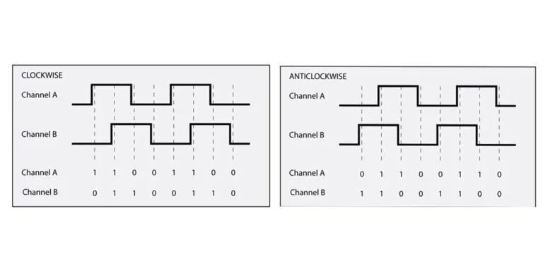
Because of the way the two signals overlap, you now have 4 signal states: 00, 01, 11, and 00. And importantly, you from any particular state, you can only go to 2 of other 3 states! For example, you cannot go directly from 11 to 00 : You must go to either 10 or 01.
Because of this, you always know what way a rotation is happening: If you're at 11, and go to 10, you're going clockwise.
This property means that quadrature encoders are much more capable than GearTooth encoders. It can still track velocity, but can measure velocities at low speeds, or with external inputs where you wouldn't know the direction.
In addition, since you always know the direction, you can also just count the pulses as they come by. This lets you know precisely how far something has rotated, effectively indefinitely.
It's important to note that another name for these is a "Relative encoder", since it only tells you a rotation relative to when it started counting! This means where your system is when the sensor starts is an important consideration!
Java Code
The WPILib Encoder classes
The Rio can directly handle external quadrature encoders using the WPI Lib Encoders classes. While uncommon in modern FRC, they show up on occasion.
Spark Encoders
Modern FRC uses brushless motors for most operations, and have built in encoders that are ready to use! As a result, this is the most common interaction with encoders.
These are accessed by interfacing with a Spark Motor controller, like so.
ExampleSubsystem extends SubsystemBase{
	//Note: Your motor ID will probably be something different!
	SparkMax motor = new SparkMax(10, MotorType.kBrushless);
	RelativeEncoder encoder = motor.getEncoder();

	// ... other stuff this way
}
If you're still getting the hang of code structure, you can work in the ExampleSubsystem.java file for now! It's all set up on new Command Based Robot templates, and will work like you're expecting.
If you're unsure about the motor ID, you can do get it using the Rev Hardware Client > Identifying a motor ID
We now have an encoder.... but it's not doing anything. Let's make it do something. Encoders are good at telling you how far they rotated, so let's print that.
ExampleSubsystem extends SubsystemBase{
	SparkMax motor = new SparkMax(10, MotorType.kBrushless);
	RelativeEncoder encoder = motor.getEncoder();

	// ... other stuff

	public void periodic (){
		System.out.println(encoder.getPosition());
	}
}
Deploy this to the robot, and you should pop up with the Riolog tab in VSCode. If not, hit CTRL+Shift+P to bring up the VS Code Command Pallete. Type "Start Riolog" to select the option, then hit enter.
You should now see a screen full of numbers. So... try rotating your motor. It should change, but it's unclear how much. We haven't configured it to any sort of a known state.
To get better diagnostic information such as graphs, or multiple values at once, you might check out Basic Telemetry
Configuring Spark Encoders
The Rev Hardware Client page can assist with adjusting parameters, which is useful for quick diagnostics and testing.
To configure it in code, we need to do a few things. First, is set up a config object, and clear factory defaults. This means we have a lot of potential quirks cleaned up instantly.
ExampleSubsystem extends SubsystemBase{
	SparkMax motor = new SparkMax(10, MotorType.kBrushless);
	RelativeEncoder encoder = motor.getEncoder();
	// ... other stuff
	public void ExampleSubsystem(){
		SparkBaseConfig config = new SparkMaxConfig();
		armMotor.configure(
			//The configuration settings to apply
			config,
			//Whether or not to reset all unspecivied values
			ResetMode.kResetSafeParameters,
			//Whether or not to keep the new values after
			//power cycling the motor controller
			PersistMode.kPersistParameters
		);
	}
	// ... other stuff
}
If you run this on your test bench, you'll probably see the numbers change differently than they did prior. By default, the encoder is configured to provide "Rotations" from the getPosition() method. If you rotate the motor shaft exactly once, the encoder will return 1.
If your testbench has some gearing involved, you'll get a different number multiplied by the gearing. For example, if you're on a Kit Of Parts drivetrain, it might have a gear ratio of 12.75:1. This means it takes 12.75 motor rotations to rotate the output wheel once. Or, put the opposite way: If you rotate drivetrain wheel exactly once, you should get an encoder reading of 12.75.
However, we generally care more about the output of the system than the motor, so we want to apply a conversion factor so we can "read" the output directly.
To get this, we need to take that logic above, and rotate our system's output exactly once. Record the number of "motor rotations" as your conversion factor, and we'll add it to the code.
ExampleSubsystem extends SubsystemBase{
	// ... other stuff
	public void ExampleSubsystem(){
		SparkBaseConfig config = new SparkMaxConfig();
		var conversionfactor=12.75; //1 divided by whatever number you determined
		config.encoder.positionConversionFactor(1/conversionfactor);
		armMotor.configure(
			config,
			ResetMode.kResetSafeParameters,
			PersistMode.kPersistParameters
		);
	}
	// ... other stuff
}
The "conversion factor" is just a multiplier from the base unit (1 rotation). Since we know that 1 output rotation generates 12.75 motor rotations, we want to divide by 12.75.
And, after we deploy this, we'll see that we can rotate our wheel once, and get an "encoder" reading of 1.
Velocity
We've been glossing over velocity, but it's time! This is helpful too. The process from this point is actually pretty easy, and we can get it with just a few minor changes.
ExampleSubsystem extends SubsystemBase{
	// ... other stuff
	public void ExampleSubsystem(){
		SparkBaseConfig config = new SparkMaxConfig();
		var conversionfactor=12.75; //1 divided by whatever number you determined
		config.encoder.positionConversionFactor(1/conversionfactor);
		//Configure the velocity conversion factor too
		config.encoder.velocityConversionFactor(1/conversionfactor/60);
		armMotor.configure(
			config,
			ResetMode.kResetSafeParameters,
			PersistMode.kPersistParameters
		);
	}
	// ... other stuff
	public void periodic (){
		//Change to velocity
		System.out.println(encoder.getVelocity());
	}
}
The main detail of note is that we use the same conversion factor to account for gearing.
We also have two ways of doing velocity conversion, depending on our desired Rate unit.
By default, 1/conversionfactor will give us Rotations Per Minute. In this case, the extra /60 is to convert from rev's default Velocity unit of Rotations Per Minute to Rotations Per Second. For many of our tasks, having the unit in "per second" winds up being more useful since it's easier to visualize.
Generally, we'll calculate the conversion factor using Position since it removes the aspect of time; This makes it much, much simpler to get accurate results.
Rotation To Linear Distance
Now that we can convert motor rotations to output shaft rotation, we can go a step further and convert that output rotation to a linear motion. This is pretty straightforward: Over 1 rotation, you cover 1 circumference of distance. So, just divide your conversion factor by your wheel diameter. Since we're calculating "x distance per rotation", so you would expect a division here.
The final configuration will look something like this:
// ... stuff
	var circumference = Math::PI * 4; // 4 inch wheel
	//1 divided by whatever number you determined
	var conversionfactor=12.75/circumference;
// ... the rest of the stuff
Managing unit conversions
If the units to configure your encoder is overwhelming, consider Factor Label methods to help you step through it. This is a useful method of tabulating units to keep track of conversions like this.
As a sample calculation, this is what it looks to set up the conversion for a KOP bot's drivetrain from motor rotations to inches per second.
| a | b | c | d | e | f | |
| 1 | motor rev | time | gear | wheel | output | |
|---|---|---|---|---|---|---|
| 2 | 1 motor rotation | 1 min | 1 output rotation | Pi * 4 inches | Cannot read properties of undefined (reading 'constructor') | ?? inch |
| 3 | minute | 60 seconds | 12.75 motor rotations | 1 output rotation | s |
Empirical analysis
Another way we'll commonly handle encoder configuration is through a simple empirical process:
- Set the encoder conversion to 1 , putting the units as "motor rotations"
- Put the system to known physical condition that's easy to measure. (zero feet traveled, arm at horizontal, etc)
- Zero the encoder (either a power cycle or a code reset)
- Move the system to a new physical condition that's also easy to measure. (10 feet traveled, arm at vertical, etc)
Keeping with our Kitbot example, in factor label form it would look something like this:
| a | b | c | d | |
| 1 | motor rev | conversion | Output | |
|---|---|---|---|---|
| 2 | 538 rotation | ??? inches | Cannot read properties of undefined (reading 'constructor') | 120 inches |
| 3 | ??? motor rotations |
Doing the math, we get
An advantage of this method is that it requires no knowledge about how a system is geared. This is great for getting a system running and validating calculations. It can also help with systems that have difficult to calculate ratios, such as winding ropes or straps.
One big disadvantage is precision: Every time you repeat this calculation, the results are slightly different. This may or may not be a problem, depending on the mechanism.
It's not advised to use empirical analysis for drivetrains! During competition, wheel wear will often force constant re-calibration. However, in pit environment it's very challenging to get space to push a drivetrain. This makes corrections time consuming and inaccurate, making your drivetrain and autos inconsistent.
Practical Applications
Having insight into the robot provides a ton of value, especially when combined with Triggers and Commands . This makes it easy to do things like
- See if a shooter is near a desired RPM before feeding a game piece into it
- See how far you've driven and stop
- Check a system's speed to see if it jammed.
We're not quite ready to do things like precisely control RPM, speed, or distance. For that, we need a PID.
Limitations and problems
Quadrature encoders are powerful, but not without flaws. The main thing is fundamental to position tracking with this type of encoder:
- You need to already know where you are when you you start counting pulses to have a meaningful knowledge of the system's position
- If something causes it to lose count (such as loss of power or a code reset), then you've lost the connection to the reference, and now don't know where you are.
There's a couple ways to avoid this. The easiest way is to start at your reference, and not lose count! As you might expect, this places some constraints on how you as humans boot up the robot. It also carries a small (but non-zero) risk for the second case.
For fully mitigating this, you need to make use of Homing Sequences , which allow you to fully recapture your reference from an unknown starting state.
Other options include simply using different sensors! For example, Absolute Encoders can capture rotation data.
To Reset or Not To Reset
Encoders all have functions to set or zero the current encoder value value. For our example, we could do this using the following code
ExampleSubsystem extends SubsystemBase{
	// ... other stuff
	public void ExampleSubsystem(){
		//Reset encoder on boot ?
		encoder.setPosition(0);
	}
	// Other stuff
But should we? We need to consider both the mechanisms physical state and the code state carefully, since we expect them to correlate. Let's examine the typical points at which one or both of these can change
- When power is applied, the mechanism is in an unknown position, the encoder is at zero, and the code runs initialization.
- When you deploy new code after running it, the mechanism can be in any state, the encoder is unchanged (by default) , and our code re-runs initialization
This leads to the following cases:
- If we power on the bot in an known reference state, the encoder will match it for the first run of code.
- If we do not reset position in initialization, we can always assert that the encoder still matches the physical position, even if we re-run or restart code.
- If we do reset position, we do so without being able to assert that we're at the hardware reference! This means we have to physically check that we're at the hardware each time manually.
Because of this, for now we probably do not want to zero the encoder, which allows us to set the physical state once on boot, and re-use it indefinitely.
If needed, you can generate Homing Sequences, which are ways for the bot to physically assert a known system state and do the reset encoders safely. These are usually optional (at least initially), but are critical for robust high-torque systems or high precision ones.
Basic Odometry+Telemetry
Synopsis
Success Criteria
- Create a Widget on a dashboard to show the field
- Populate the Field with your robot, and one or more targets
- Utilize the Field to help develop a "useful feature" displayed on the Field
As a telemetry task, success is thus open ended, and should just be part of your development process; The actual feature can be anything, but a few examples we've seen before are
- showing which of several targets your code has deemed best, and react to it
- a path your robot is following, and where the bot is while following it
- The current Vision targets and where your bot is when seeing them
- A field position used as an adjustable target
- The projected path for a selected auto
- Inidcate proximity or zones "zones" for performing a task, such as the acceptable range for a shooting task or intaking process.
Odometry Fundamentals
Odometry is also known as Position Tracking. In FRC, this is generally regarded as knowing the position of your robot in the game field. It is most beneficial when combined with the robot to then have the robot move between positions on the field, and interact with other known positions.
Actually obtaining odometry depends on the design of the bot: Differential Drive Odometry or Swerve Odometry , and often involves vision systems via LimeLight Odometry or PhotonVision Odometry
This document is concerned with the prerequisite: Being able to actually view, compare, and validate positions using robot telemetry.
Odometry Telemetry
Telemetry for Odometry revolves around the Field2D object. Both Glass and Elastic can display the Field2D object as a game field on the dashboard, including associated robot positions and any secondary objects.
In general, Glass is the superior option for most programming tasks and development, allowing easier customization to help reduce clutter and provide clarity between objects.
The WPILib Docs are excellent at helping demonstrate many of these examples:
https://docs.wpilib.org/en/stable/docs/software/dashboards/glass/field2d-widget.html
Pose
In Robots, a Pose represents a specific location and state of a robot's actuator. Within the context of odometry, a pose represents the robot's location on a 2D plane. In most cases, this means the location on the game field.
In order to represent such a state, we need 3 things: The X position, the Y position, and a rotation.
In WPILib, this is handled by the Pose2d object, which can be provided to and returned from many utilities interacting with the robot position, including drivetrain path planning, vision, simulation, and telemetry.
Field2D Basics
The Field2D object in WPILib contains a number of utilities for keeping tabs on odometry. It can be added with just a couple lines.
class Drivetrain extends SubsystemBase{
	Field2D field = new Field();

	public Drivetrain(){//constructor
		//We only want to send the actual Field object _once_,
		//so we often do it in the constructor. Changes will be
		//sent automatically as the Field2d object itself is updated.

		//Preferred: Set the NetworkTables name explicitly,
		//and give it a unique, descriptive name
		SmartDashboard.putData("ChassisField",field);

		// This form uses the default name "Field" as the key.
		// Not recommended in most cases
		//SmartDashboard.putData(field);
	}

}
This creates a blank, empty field, with your robot position, probably at (0,0) in the bottom left corner, on the blue side of the field.
Meaningfully updating the robot pose is out of scope, and differs by drivetrain type; However, the basic gist is
class Drivetrain extends SubsystemBase{
	Field2D field = new Field();
	//Set up an odometry object to track our robot
	DifferentialDrivePoseEstimator odometry=new DifferentialDrivePoseEstimator(
	 /* Complex constructor parameters; not relevant*/
	)

	public Drivetrain(){//constructor
		SmartDashboard.putData("ChassisField",field);
	}

	public void periodic(){
		//Read the odometry object and set the pose. //Reference only
		field.setRobotPose(odometry.getPoseMeters());

		// Or, we can just set it manually for testing.
		field.setRobotPose(new Pose2d(2.7,3.1, new Rotation2d(Math.PI/2.0) ));
	}
}
Now, when we open our Field2D widget in Glass, we'll see that our robot is at a new position. If we fully implemented our Pose Estimator object, we'd see that this provides realtime tracking of our position.
A .getRobotPose() also exists, but tends to be less useful in practice, as most classes that will interact with the Robot and Field will likely have access to the Odometry object directly.
Note, that the Field2d object we create is a unique reference, with it's own unique local data; only the NetworkTables key might have overlap when using default keys. This means if we want to properly share a Field across multiple classes, we either need to fetch the NetworkTables data and copy it over, create a single Field object in RobotContainer and pass it to, or create a DriverField object as a Singleton that can facilitate a single object.
Displaying Useful Targets
Where Field2d objects really shine is in adding supplemental information about other field objects. The utility varies by game, but it's great for showing a variety of things such as
- Targets/objectives
- Nearest/best target
- Nearest game piece (detected by vision systems)
These can be done using the getObject(name) method; This grabs the named object from the field, creating it if it doesn't already exist.
class Drivetrain extends SubsystemBase{
	Field2D field = new Field();

	public Drivetrain(){//constructor
		SmartDashboard.putData("ChassisField",field);
	}

	public void periodic(){
		//Can provide any number of pose arguments
		field.getObject("GamePieces").setPoses(
			new Pose2d(1,1),
			new Pose2d(1,2),
			new Pose2d(1,3),
		);
		//You can also pass a single List<Pose2d>
		//if you have a list of poses already

		field.getObject("BestGamePiece").setPose(
			new Pose2d(1,2)
		);
	}

}
Note It's worth considering that for objects that never move, you could set objects once in the constructor, and they work fine. However, if the user accidentally moves them in the UI, it creates a visual mis-match between what the code is doing and what the user sees. As a result, it's often better to just throw it in a Periodic.
Field2d + User Input
A niche, but very useful application of field objects is to get precise driver feedback on field location data. This can be done using the following code setup:
class Drivetrain extends SubsystemBase{
	Field2D field = new Field();

	public Drivetrain(){//constructor
		SmartDashboard.putData("ChassisField",field);
		//Set the pose  exactly once at boot
		field.getObject("DriverTarget").setPose(
			new Pose2d(1,2)
		);
	}

	public Command aimAtCustomTarget(){
		return run(()->{
			var target=field.getObject("DriverTarget").getPose();
			//Do math to figure out the angle to target
			//Set your drivetrain to face the target
		};
	}

	public void periodic(){
		//No setting DriverTarget pose here!
	};
}
In this case, we take advantage of the "set once" approach in constructors; The drivers or programmers can modify the position, and then we now read it back into the code.
This can be very useful for testing to create "moving targets" to test dynamic behavior without having to drive the bot. It can also help you create "simulation" poses for testing math relating to Pose2D objects.
is especially true for simulation, as this allows you quickly test pose-related functions and makes sure that things happen how you expect.
One practical application is match-specific targets for cooperating with allies. An example is in 2024 Crescendo: a common game tactic was to "pass" rings across the field, by shooting to an open area near where your allies would be. However, since the game pieces can get stuck in/on robots, and different robots have different intakes, and each ally has different sight lines, making the ideal pass target unknown until the actual match is about to start. An adjustable target let the alliance sort it out before a match without having to change the code.
Displaying Paths
When doing path-planning for drivetrains, it's often helpful to display the full intended path, rather than a lot of individual poses.
class Drivetrain extends SubsystemBase{
	Field2D field = new Field();

	public Drivetrain(){//constructor
		SmartDashboard.putData("ChassisField",field);
		//Set the pose  exactly once at boot
		field.getObject("DriverTarget").setPose(
			new Pose2d(1,2)
		);
	}

	public Command buildAuto1(){
		var  trajectory=// Get the trajectory object from your path tool
		field.getObject("autoTrajectory").setTrajectory(trajectory);
		return run(()->{
			//draw the rest of the owl
		};
	}


}
In this use case, the work will likely be done inside your Auto class after selecting the appropriate one.
Robot Code Basics
Success Criteria
- Install the WPILib VS Code IDE
- Make a new robot project
- Create a new subsystem
- Install the Rev third Library
- Basic requirements to start working on robot projects
- Create a new empty subsystem
- Create a new empty command
- Add your new command and subsystem to RobotContainer.
Goals
Programming prerequisites, listed in Coding Basics for now
Robot Code structure
When you open a new robot project you'll see a lot of files we'll interact with.
src/maindeployjavafrc/frc/robotcommandsExampleCommand.java
subsystemsExampleSubsystem.java
Constants.javaMain.javaRobot.javaRobotContainer.java
vendordeps
For typical projects, you'll be spending the most time in RobotContainer, subsystems, and occasionally commands.
For some early practice projects, or special use cases you might also interact with Robot.java, ExampleCommand.java, or ExampleSubsystem.java a bit.
Third Party Libraries
Many helpful utilities we'll use for robot projects are represented using code that's not available by default. WPILib has a small manager to assist with installing these, detailed here:
Third Party Tools
We'll also utilize a number of software tools for special interactions with hardware or software components. Some of these include
- Rev Hardware Client , a motor controller management tool
- GrappleHook , which manages the LaserCan configuration
- NI Driver Station is needed for systems that will want to enable and drive a robot.
Putting Things in the Proper Place
The hardest part of getting started with robots is figuring out where your robot code goes.
Robot.java : A microcausm of the complete robot
Robot.java is a very powerful file, and it's possible to write your entire robot in just this one file! For reasons we'll get into later, we do not want to do this. However, the setup of it does a good job explaining how a robot works. Let's look at the structure of this file for now
public class Robot extends TimedRobot {
	private Command m_autonomousCommand;
	private final RobotContainer m_robotContainer;
	public Robot() {
		m_robotContainer = new RobotContainer();
	}

	public void robotPeriodic() {}

	public void disabledInit() {}
	public void disabledPeriodic() {}

	public void autonomousInit() {}
	public void autonomousPeriodic() {}

	public void teleopInit() {}
	public void teleopPeriodic() {}

	public void testInit() {}
	public void testPeriodic() {}

	//a few more ignored bits for now
}
From the pairing, we can group these into several different modes
- "Robot"
- Autonomous
- Teleop
- Test
Indeed, if we look at our Driver Station, we see several modes mentioned.
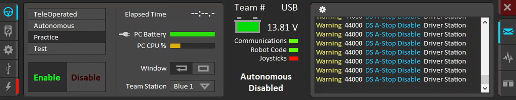
Teleop, Auto, and Test are simply selectable operational modes. However, you might want to utilize each one slightly differently.
"Practice mode" is intended to simulate real matches: This DriverStation mode runs Autonomous mode for 15 seconds, and then Teleop Mode for the remainder of a match time.
"Disabled" mode is automatically selected whenever the robot is not enabled. This includes when the robot boots up, as well as as whenever you hit "disabled" on the driver station.
Disabled mode will also cancel any running Commands .
"Robot mode" isn't an explicit mode: Instead, of "Robot Init", we just use the constructor: It runs when the robot boots up. In most cases, the primary task of this is to set up Robot Container.
robotPeriodic just runs every loop, regardless of what other loop is also running.
We can also see a grouping of
- Init
- Periodic
Whenever any new "mode" starts, we first run the Init function once, and then we run the periodic. The robot will continue run associated Periodic functions every loop, 50 times per second.
We generally won't add much code in Robot.java, but understanding how it works is a helpful starting point to understanding the robot itself.
RobotContainer.java
As mentioned above, the "Robot Container" is created when you create a new project, and one of the first things that gets executed when running robot code.
This file contains a small number of functions and examples to help you organized.
public class RobotContainer(){
	ExampleSubsystem subsystem = new ExampleSubsystem();
	ExampleCommand command = new ExampleCommand();
	CommandXboxJoystick joystick = new CommandXboxJoystick(0);
	RobotContainer(){
		configureBindings();
	}
	public void configureBindings(){
		//Not a special function; Just intended to help organize
	}
	public Command getAutonomousCommand(){/*stuff*/}
}
This file introduces a couple new concepts
- Commands, which form the "actions" you want the robot to perform
- Subsystems, or the different parts of the robot that could perform actions
- Joysticks , which serve as the standard input method.
The use of Commands and Subsystems goes a long way to managing complex robot interactions across many subsystems. However, they're certainly tricky concepts to get right off the bat.
Constants.java
Sometimes, you'll have oddball constants that you need to access in multiple places in your code. Constants.java advertises itself as a place to sort and organize these constants.
Without getting too into the "why", in general you should minimize use of Constants.java; It often leads to several problems as your robot complexity increases.
Instead, keep your constants as close to where they're used as possible, and move them up through the robot hierarchy as necessary. This is known as "scope management" or "encapsulation".
- If a value is used once, just use the value directly. This covers a lot of setup values like PID tuning values.
- If your value is used repeatedly inside a subsystem, make it a private constant in that subsystem. This is common for conversion factors, min/max values, or paired output values
- If a constant is strongly associated with a subsystem, but needs to be referenced elsewhere, make it a public constant in that subsystem.
- Lastly, if something is not associated with a subsystem, and used repeatedly across multiple subsystems, Constants.java is the place.
If you find yourself depending on a lot of constants, you might need to consider Refactoring your code a bit to streamline things. Note that Stormbots code generally has almost nothing in here!
ExampleSubsystem.java
The ExampleSubsystem.java file is a preconfigured, blank Subsystem. We'll explore Subsystems in depth later.
By default, this class is created, and the periodic() function it contains will run every code loop. This makes it a great place to put a lot of starter code with minimal setup and fuss.
ExampleCommand.java
This is a standard, blank Command . By itself, this file is not too useful. However, the fact that it exists allows useful joystick interactions to be set up in RobotContainer.java
Understanding The Examples
The code examples provided in early code samples will be built using ExampleSubsystem and ExampleCommand, built into every new robot project. They should work as expected without a deeper understanding of Command based robots while you get your footing, and enabling you to migrate to Command based robots once you get there. If an example doesn't talk about Command based stuff, you probably don't have to worry about it!
Creating new files
While you can just create new files in a "normal" way, it's easy to accidentally miss code details that make things harder for yourself.
Instead, WPILib+VSCode has a built in way to do this. Simply right click the appropriate folder, and find the "Create new class/command" option.
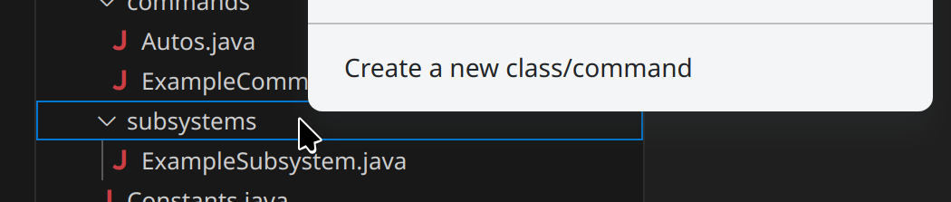
This will present you with a list of common FRC classes. The typical ones you'd use are Command and Subsystem.
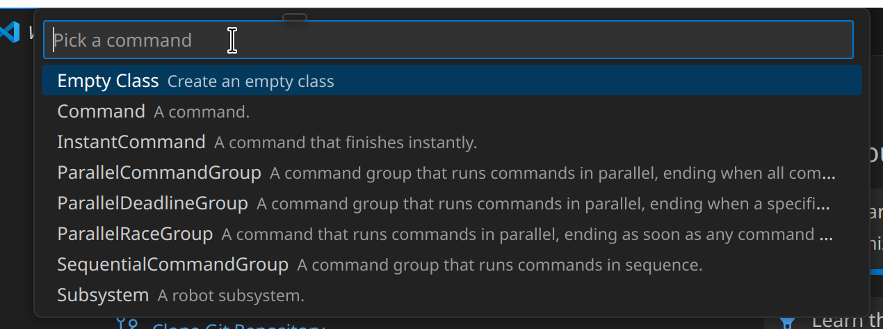
Code Flow
For those familiar with coding, you might wonder "Where does code actually start from?". This is a fair question in FRC code, which is a more complicated framework. The code path itself is predictable and a simplified view looks like this
- Main Bot Initialization
  - Robot.java::RobotInit
    - RobotContainer
      - Subsystem Constructors
      - Command constructors
  - Enter Disabled mode

- Disabled Mode
  - Initialize
    - Robot.java::DisabledInit()
  - Loop
    - Robot.java::DisabledPeriodic
    - (each subsystem)::periodic()

- Teleop Mode
  - Initialize
    - Robot.java::TeleopInit()
    - (any active commands)::init()
  - Loop
    - Robot.java::TeleopPeriodic()
    - (each subsystem)::periodic()
    - (any active commands)::execute()
This is a lot of complexity if you're new to coding, but don't panic. You can mostly ignore a lot of this complexity, and our examples will help you position things properly until you get your bearings.
The complex part, robot actions that move motors and do things, basically boil down into
initialize/prep on boot
disabled
initialize
run
stop
We will quickly capture this with our Commands framework, enabling you to do simple things very quickly and efficiently, like they're self-contained little programs.